Capital Market Expectation - CME

Framework and Macro Considerations

• Economic Forecasting - Econometric Analysis

  • Structural Model: based on economic theory 有理论

  • Reduced-form: might be without theory, base on data and correlation 无理论支撑，数据之间的关系 regression

  • Pros and Cons

  • Pros:

    1. Many factors,

    2. Quantitative,

    3. Has a model, so can easily generate output,

    4. Discipline consistency

  • Cons:

    1. Complex and Time-consuming

    2. Data input might be hard to forecast

    3. Model is static, model might be mis-specified. Model is based on past data, so the model is static, cannot be updated while the market regime changed 因为模型基于过去数据，所以模型是static的，不能随市场情况更新

    4. False sense of precision 模型model cannot forecast future well

    5. Not forecast turning points 无法或者滞后的预测turning points

• Indicators 用 indicator 预测经济情况

  • Leading indicators. A composite of leading indicators is called a diffusion index

  • Pros and Cons

    • Pros:

      1. Simple,

      2. Could forecast turning points

      3. Easy to Track, good availability of indicator data

    • Cons:

      1. Time lag滞后, revised指标可能修正, rebased基期变化

      2. 单一指可能给出 false signals

      3. 多个指标可能结果不一致，no binary guidance

• Checklist Approach 问卷调查

  • Pros:

    1. Simple

    2. Flexible 咋问都可以

• Cons:

  1. Subjective 主观

  2. Time Consuming

  3. Manual Process limits depth analysis

  4. No consistency of analysis

Challenges in Forecast

1. Limitations to using economic data

   • 数据 revised / rebased

2. Data measurement errors and biases

   • Transcription errors 抄错了

   • Survivorship bias. The survivorship bias might overestimate returns 如PE知有表现好的时候才公布收益，所以 survivorship bias 高估 return

   • Appraisal data. The higher the frequency of data, the lower the correlation, because data become no smoothy. Lower the correlation, higher the risks 数据频率越高，corr越低（因为assume 高频数据是大幅波动的，所以corr低），则 risk 越低。 Return smoother biases downward the risks

3. Limitations of historical estimates

   • Regime changes make data non-stationary. 由于 regime changes，造成 data non-stationary

   • Non-stationary make data statistically non-predictable.

   • Long time period & large dataset are preferable. Asynchronous data (high frequency data) underestimate correlation and underestimate risks.

4. Ex-post (将来) risk as a biased risk measure ex-ante (过去的) risk

   • 站在将来看过去 underestimate the risks and overestimate the potential returns

5. Biases in Analyst's Methods

   • Data-mining 相关性不代表因果关系

   • Time-period Bias 时间选太长会有 regime changes，太短 asynchronous data会导致 low corr， low risks

   • Avoid Bias:

     1. data has economic basis, 数据有经济含义 ，避免相关性因果关系的问题

     2. Scrutinty 仔细检查 examine and inspect closely and thoroughly

     3. Test relationship with out-of-sample data 用样本外数据建议

6. Prudence Trap: The prudence trap is the tendency to be cautious when making decisions that could be potentially expensive or damaging to the decision maker’s career.

Economic Growth

Exogenous Shocks (unanticipated)

Factors cause the exogenous shocks

• Changes in Government Policy

• Political Events

• Technological progress

• Natural disasters

• Discovery of natural resources

• Financial crisis

Application 预测 $r_e$$r_e$ Equity Return

$r_e=\frac{D_1}{P_0}+g_{equity}$$r_e = \frac{D_1}{P_0} + g_{equity}$

By Golden Growth Model: $P_0=\frac{D_1}{r_e-g}$$P_0 = \frac{D_1}{r_e-g}$, we expand that into the whole equity market, that $r_e=\frac{D_1}{P_0}+g$$r_e = \frac{D_1}{P_0} + g$

1. $\frac{D_1}{P_0}$$\frac{D_1}{P_0}$

$\frac{D_1}{P_0}=\frac{D_1/EPS}{P_0/EPS}=\frac{DivPayoutRatio}{P/Eratio}$$\frac{D_1}{P_0} = \frac{D_1 / EPS}{P_0/EPS} = \frac{Div\ Payout\ Ratio}{P/E\ ratio}$

2. $g_{equity}$$g_{equity}$

• Normal GDP Growth

  Growth or Shocks might be reflected into stock price and bond price.

  Growth 大 => inflation 大 => tight monetary policy ( r 提升 => yield 提升 => bong price下降

  $P_1=GD{P}_1\times \frac{E_1}{GD{P}_1}\times \frac{P_1}{E_1}$$P_1 = GDP_1 \times \frac{E_1}{GDP_1}\times \frac{P_1}{E_1}$

  • $P_1$$P_1$: stock price

  • $E_1$$E_1$: earning

  • $P_1$$P_1$: Price

  • $S_1$$S_1$: (%) shares of Earning / GDP

  Price_1 = Total Economy * S_1 * 市盈率

  $\frac{P_1}{P_0}=\frac{GD{P}_1}{GD{P}_0}\times \frac{E_1/GD{P}_1}{E_0/GD{P}_0}\times \frac{P_1/E_1}{P_0/E_0}$$\frac{P_1}{P_0} = \frac{GDP_1}{GDP_0} \times \frac{E_1/GDP_1}{E_0/GDP_0} \times \frac{P_1/E_1}{P_0 / E_0}$

  $ln(\frac{P_1}{P_0})=ln(\frac{GD{P}_1}{GD{P}_0})+ln(\frac{E_1/GD{P}_1}{E_0/GD{P}_0})+ln(\frac{P_1/E_1}{P_0/E_0})$$ln(\frac{P_1}{P_0}) = ln(\frac{GDP_1}{GDP_0}) + ln( \frac{E_1/GDP_1}{E_0/GDP_0}) + ln(\frac{P_1/E_1}{P_0 / E_0})$

  Stock price growth = GDP growth + S growth + P/E ratio Growth

  $g_{equity}=g_{gdp}+\mathrm{\Delta }S\mathrm{\%}+\mathrm{\Delta }P/E\mathrm{\%}$$g_{equity} = g_{gdp} + \Delta S\% + \Delta P/E \%$

  • Short-term 三项都变

  • Short-term 只有 growth of GDP 变, so $g_{equity}=g_{GDP}$$g_{equity} = g_{GDP}$

• Real GDP Growth $Y=\frac{Y}{L}\times L$$Y = \frac{Y}{L} \times L$

  Real GDP = GDP per Capita * Labour

  L 劳动力规模 has two drivers: (1) growth in potential labour force size, (2) labour force participation.

  Y/L productivity 劳动力效率 has two drives: (3) capital inputs (4) TFP total factor productivity

3. Thus, in the long term

   Long-term: $g_{equity}=g_{nominalGDP}=g_{real}+\pi$$g_{equity} = g_{nominalGDP } = g_{real} + \pi$

   $g_{realGDP}=(1)+(2)+(3)+(4)$$g_{real GDP} = (1) + (2) + (3) + (4)$

   Short-term: $g_{equity}=g_{gdp}+\mathrm{\Delta }S\mathrm{\%}+\mathrm{\Delta }P/E\mathrm{\%}$$g_{equity} = g_{gdp} + \Delta S\% + \Delta P/E \%$

Business Cycle

Reason of cyclical business activities

• imperfect information to make decision

• reversing incorrect decision can be costly

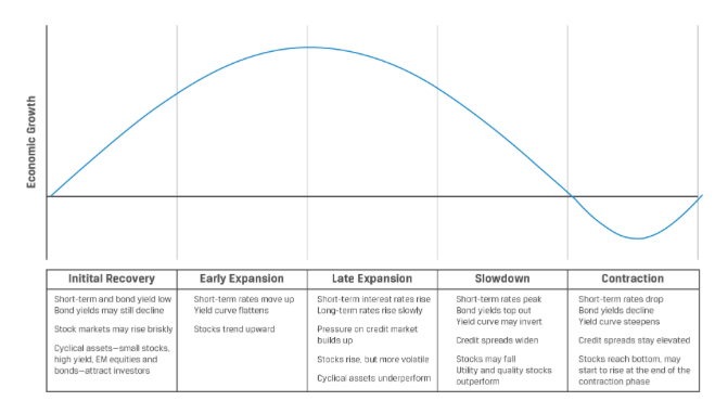
Phases

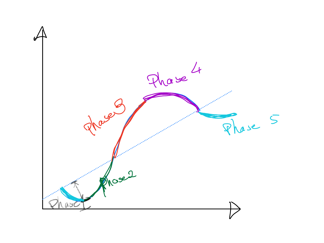
• short-term rate by CB is same as the slope of curve

  • bond price is negative corr with short-term rate

  • short-term rate 代表 economic policy 强度

• Inflation lags with the short-term rate 通胀滞后于short-term rate

• output gap is the diff between potential GDP & actual

1. Initial Recovery 复苏期

• Gov stimulate the econ by lower interest, increease budget deficits.

  • Falling interest rate

• Falling inflation

• Negative output gap: Actual GDP < Potential GDP

• stock price increasing

• Buy: risky assets such as small-cap stocks and high-yiedl bonds

2. Early Expansion 早期成长

• still low inflation

• increase in confidence

• Short-term rate increasing

  • bond yield increase, so bond price decrease

• output gap narrows

• Buy: stocks

3. Late Expansion

• high confidence and high employment

• No Output Gap: Actual GDP > Potential GDP

• CB reduce the growth of Money Supply (restrictive monetary policy)

  • Short-term rate increasing

  • bond yield increase, so bond price decrease

  • stock price achieve the top, sell stocks

4. Slowdown

• Inflation still Increase

• Short-term rate Peak (achieve the peak, and going down 在4的最开始 curve flat -> achieve the top)

  • bond yield peak, bond price goes to the bottom

• Might have inverted yield curve, short-term rate > long term rate

• Buy: Bond as it achieves the bottom

5. Contraction

• Low confidence and profits, low employment

• inflation top out

• Short-term rate faills

  • bond yield falls

• Stock price achieve the bottom at the end of recession, so buy stock then

Inflation

• Dis-inflation: means inflation decrease, i.e. from 8% to 5%. Dis-inflation migh decelerate the econ. 但是因为inflation 下降了，但 还是正的，price还在提升

• Deflation: negative inflation 是负的

Deflation is worst! in that, while asset price decrease (deflation), the balance sheet ends up with negative equity. Borrower cannot repay the interests, then Default!

1. Default on Debt Obligations

2. Monetary Policy not working, coz inflation negative drives interest rate negative.

   • QE to stimulste the econ

   • however, QE is working in the U.S. because the state of USD, but normally unable to work in other countries, such as CN and JP

Buy

• Inflation within expectations: 买 stock, inflation is reflected into the stock price

  1. Cash equivalents: Earn the real rate of interest

  2. Bonds: Shorter-term yields more volatile than longer-term yields

  3. Equity: No impact given predictable economic growth (已经反映在预期中 )

  4. Real estate: Neutral impact with typical rates of return

• Inflation above or below expectations: 买 固定资产 real estate 保值，保持购买力

  1. Cash equivalents: Positive (negative) impact with increasing (decreasing) yields

  2. Bonds: Longer-term yields more volatile than shorter-term yields

  3. Equity: Negative impact given the potential for central bank action or falling asset prices, though some companies may be able to pass rising costs on to customers

  4. Real estate: Positive impact as real asset values increase with inflation

• Deflation: 资产价值降低，Fixed-income 保持收入(if no default), cash keeps its value. 所以不买 stock 买 high-rated bond + cash

  1. Cash equivalents: Positive impact if nominal interest rates are bound by 0%

  2. Bonds: Positive impact as fixed future cash flows have greater purchasing power (assuming no default on the bonds)

  3. Equity: Negative impact as economic activity and business declines

  4. Real estate: Negative impact as property values generally decline

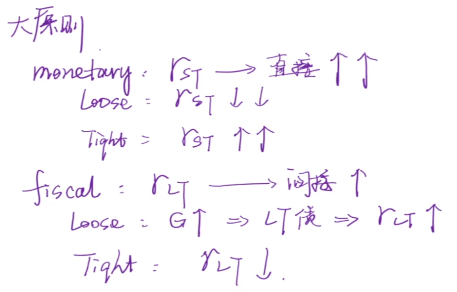
Policy Impacts

Monetary Policy

• Taylor Rules

  $r_{policy}=r^{\ast }+\frac{1}{2}(\pi -{\pi }^{\ast })+\frac{1}{2}(Y-Y^{\ast })$$r_{policy } = r^* + \frac{1}{2} (\pi-{\pi}^*) +\frac{1}{2}(Y-Y^*)$

• Negative Interest Rate 负利率情况下

  • few comparable periods, 因为 negative interest rate 的历史数据样本小，所以用历史数据估计未来，估计不准确

  • it means significant structural changes

  如何处理负利率的情况？

  1. 用 neutral rate 替代负利率

  2. 不处理

Fiscal Policy

• Consider the changes in the budget deficits, not absolute value.

• Crowding out Effects: rising public sector spending drives down or even eliminates private sector spending.

• Automatic Stabliser:

  1. Progressive Tax:

     Expansion => Income increase => tax increase => consumption decrease

  2. Mean-based transfer payment 转移支付

     recession => transfer payment 补贴 => consumption increase => stimualte the econ

Monetary + Fiscal Policy

$i=\pi +r$$i = \pi + r$

• Monetary Policy 影响 $\pi$$\pi$ , inflation

• Fiscal Policy 影响 $r$$r$ , real interest rate

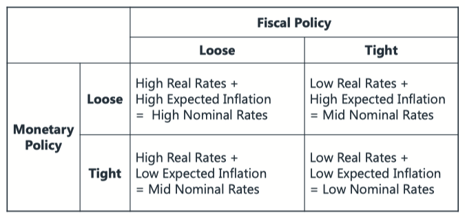
Impacts on Yield Curve

• If both policies are stimulative, the yield curve is steep and the economy is likely to grow.

• If both policies are restrictive, the yield curve is inverted and the economy is likely to contract.

• If monetary policy is restrictive and fiscal policy is stimulative, the yield curve is flat and the implications for the economy are less clear.

• If monetary policy is stimulative and fiscal policy is restrictive, the yield curve is moderately steep and the implications for the economy are less clear.

International Consideration

If Current Account Surplus, => Net Export (export > import), => capital inflow 资本流入（钱流入国内）foreign reserve increase 外储增加, => 用外储USD投资海外资产 => 资本外流 => Capital Account Deficits

反之

If Current Account Deficits, Import > Export, 需要借外汇来进口, Capital Account inflow (Surplus)

• Therefore, Current Account & Capital Account negative correlated

Interest Rate/Exchange Rate Linkages

$Y=C+I+G+NX$$Y = C+I+G +NX$

$NX=Y-C-I-G$$NX = Y-C-I-G$

by $Y-T=C+S$$Y-T = C+S$, so $Y-C=S+T$$Y-C = S+T$

Thus, $NX=\underset{\text{Net Private Saving}}{\underbrace{S-I}}+\underset{\text{Government Surplus}}{\underbrace{T-G}}$$NX = \underbrace{S-I}_{\text{Net Private Saving}} + \underbrace{T-G}_{\text{Government Surplus}}$

Peg 一国汇率peg另一国

• The linkage between the business cycles of the two economies will increase, as the pegged currency country must follow the economic policies of the country to which it has pegged its currency. 两国的经济政策必须一致，否则peg不住

• The interest rates of the pegged currency will exceed the interest rates of the currency to which it is linked, and the interest rate differential will fluctuate with the market’s confidence in the peg. 利差会导致peg不住

不可能三角

• Unrestricted Capital Flow 自由的资本流动

• Fixed Exchange Rate

• Independent Monetary Policy

Text Sample: Eastland currently has a fixed exchange rate pegged to Northland with unrestricted capital flows. Eastland is unable to pursue an independent monetary policy with interest rates in Eastland equal to the interest rates prevailing in Northland (the country to which the currency is pegged). If Eastland allows the exchange rate to float, it will now be able to run an independent monetary policy with interest rates determined in its domestic market.

Forecast Asset Class Return

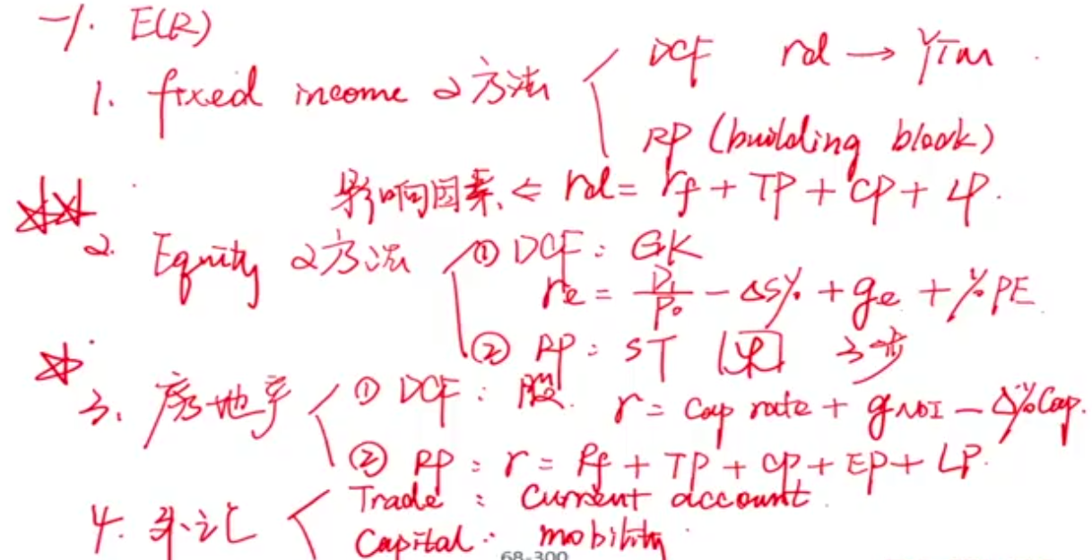
Fixed Income

DCF Approach

$P_0=\sum \frac{C{F}_t}{(1+r{)}^t}$$P_0 = \sum \frac{CF_t}{(1+r)^t}$

• $r=YTM$$r = YTM$, there are three assumption about YTM, 只要违背这三个assumption，那么估值不准确

  1. Hold to Maturity 持有至到期

  2. No Default 不违约

  3. reinvest at YTM 以 YTM 的 rate 再投资

• $r=\text{coupon rate}+\text{Re-Investment}+\mathrm{\Delta }P$$r = \text{coupon rate} + \text{Re-Investment} + \Delta P$

  • if market rate increase,

    1. then $\mathrm{\Delta }P$$\Delta P$ decrease. => Price Risks increase

    2. $RI$$RI$ increase. 再投资 CF 的收益提升 => re-investment risks decrease

    • vice versa

  • Duration Gap = "MI" = Maculy Duration - Investment Period

    • if DG > 0, Maculy Duration is larger, price risks dominates. Thus, market rate increase, impacts of $\mathrm{\Delta }P$$\Delta P$ > impacts of $RI$$RI$, => thus $r$$r$ increase, bond price decreases.

Risk Premium Approach

$r=r_f+TP+CP+LP$$r = r_f + TP + CP + LP$

= Rf + Term Premium + Credit Premium + Liquidity Premium

• risk free rate: short term 因为如果是长期的就不需要 term premium, similarly risk-free rate without TP CP LP risks

  • T-bill rate, if negative interest rate, then use policy rate replaced

  • if term is mismatched 如果期限错配, use Future Contract Rate (forward rate, or future rate)

• Term premium

  1. Inflation Uncertainty

     The term structure is positively correlated with inflation uncertainty

     $TP=r_{longTerm}-r_{shortTerm}$$TP = r_{longTerm} - r_{shortTerm}$

  $STinflation:i=\theta$$ST \ inflation: i = \theta$ <- expected inflation

  $LTinflation:i=\theta +\pi$$LT\ inflation: i = \theta + \pi$ <- expected inf + uncertainty inf

  $r_{LT}=l+\theta +\pi$$r_{LT} = l + \theta + \pi$ real interest rate + inflation

  $r_{SL}=l+\theta$$r_{SL} = l + \theta$ real interest rate + inflation

  $TP\sim \pi$$TP \sim \pi$

  2. Recession Hedge

     衰退 -> buy T-bond -> long-term bond price increase -> $r_{LT}$$r_{LT}$ decrease

     $TP=r_{LP}-r_{ST}$$TP = r_{LP} - r_{ST}$ decrease

  3. Supply and Demand

     Long-term bond demand > supply, price incerase, $r_{LT}$$r_{LT}$ decrease

     $TP=r_{LP}-r_{ST}$$TP = r_{LP} - r_{ST}$ decrase

  4. Business Cycles: Slope of the yield curve

• Credit premium

  1. Expected Loss = PD * LGD <- Prob of Loss * Loss Given Default

     LGD increase -> CP increase

  2. Default Risks: Default Risks increase increase, CP increase

  3. Credit Rating: Low Credit Rating -> high credit premium

  • Empirical Finding: Default Risk has the majority among those three

• Liquidity premium

  the LP is higher if the bonds are:

  1. issued at close to par or market rates,

  2. new,

  3. large in size,

  4. issued by a frequent and well-known issuer,

  5. simple in structure, and

  6. of high credit quality.

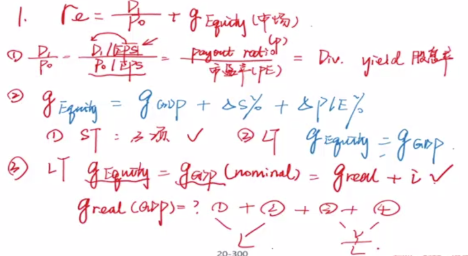
Equity Return

GK model (DCF) - Supply Side (from the firm side) Grinold and Kroner Model

GGM -> 3 steps -> GK model

$GGM:r_e=\frac{D_1}{P_0}+g$$GGM: r_e = \frac{D_1}{P_0}+g$

• Step 1: Expected Cash Flow Returns 调 share changes，$+\mathrm{\%}\mathrm{\Delta }S$$+\% \Delta S$

• if it is the Repurchase, then there shall be a minus sign. $-\mathrm{\%}\mathrm{\Delta }S$$-\% \Delta S$

  因为 Dividend Yield: Cash Div + Share changes (Repurchase)

  其中回购越多，对 shareholders 越好，因为 share 被浓缩了，同时因为 $\mathrm{\%}\mathrm{\Delta }S$$\% \Delta S$ 本身是负数，所以

  调增为 $+\mathrm{\%}\mathrm{\Delta }S$$+\% \Delta S$

• Step 2: The Expected Nominal Earning Growth $\mathrm{\%}\mathrm{\Delta }E$$\%\Delta E$

  $\mathrm{\%}\mathrm{\Delta }E=g_{real}+\pi$$\%\Delta E = g_{real} + \pi$ , real growth + inflation

  we use the nominal earning growth of the firm, not the country

• Step 3: Repricing Return: $\mathrm{\%}\mathrm{\Delta }P/E$$\% \Delta P/E$

• Thus,

  • $r_e=\frac{D_1}{P_0}+(-)\mathrm{\%}\mathrm{\Delta }S+\mathrm{\%}\mathrm{\Delta }E+\mathrm{\%}\mathrm{\Delta }P/E$$r_e = \frac{D_1}{P_0} +(-) \%\Delta S + \%\Delta E + \%\Delta P/E$

  • $r_e=\frac{D_1}{P_0}+(-)\mathrm{\%}\mathrm{\Delta }S+g_{real}+\pi +\mathrm{\%}\mathrm{\Delta }P/E$$r_e = \frac{D_1}{P_0} +(-) \%\Delta S + g_{real} + \pi + \%\Delta P/E$

• P.S. Sample Text: Grinold–Kroner model states that the expected return on equity is the sum of the expected income return (2.4%), the expected nominal earnings growth return (7.3% = 2.3% from inflation + 5.0% from real earnings growth) and the expected repricing return (−3.45%). The expected change in market valuation of −3.45% is calculated as the percentage change in the P/E level from the current 14.5× to the expected level of 14.0×: (14 − 14.5)/14.5 = −3.45%. Thus, the expected return is 2.4% + 7.3% − 3.45% = 6.25%.

  • Expected Cash Flow (Income) Return = $D/P+(-)\mathrm{\%}\mathrm{\Delta }S$$D/P +(-) \%\Delta S$

  • Expected Nominal Earnings Growth Return = $\mathrm{\%}\mathrm{\Delta }E$$\%\Delta E$ (Inflation + Real Earning Growth)

  • Expected Repricing Return = $\mathrm{\%}\mathrm{\Delta }P/E$$\%\Delta P/E$

Pros and Cons

• Pros: 考虑了 (1) Repurchase, (2) Nominal Growth, (3) Repricing Return

• Cons: the model assume infinite time horizon

  • coz in the long run, $\mathrm{\%}\mathrm{\Delta }P/E=0$$\%\Delta P/E = 0$ and $\mathrm{\%}\mathrm{\Delta }S=0$$\%\Delta S =0$

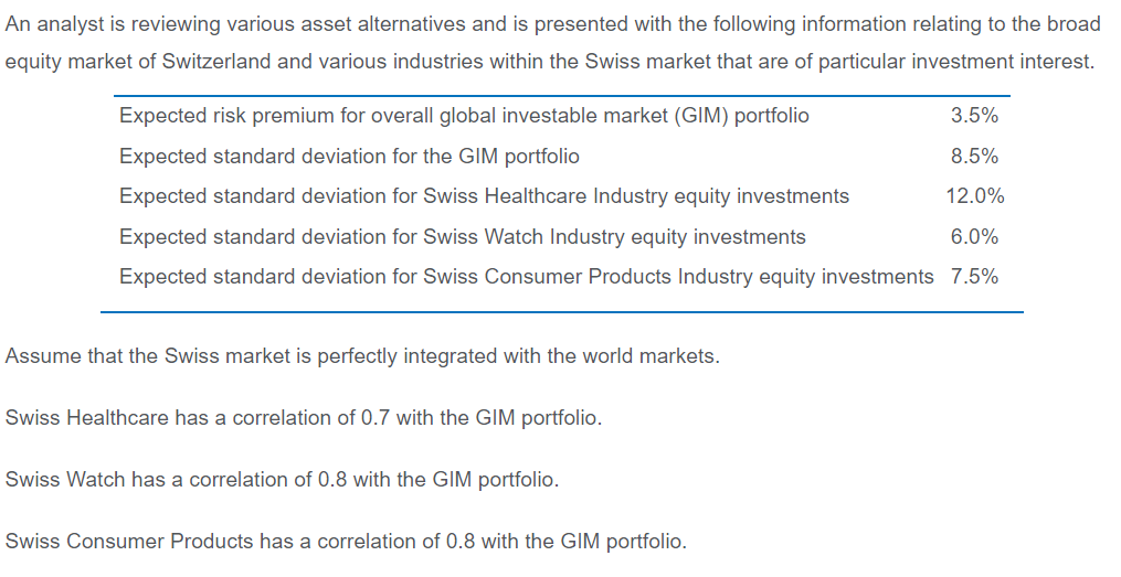
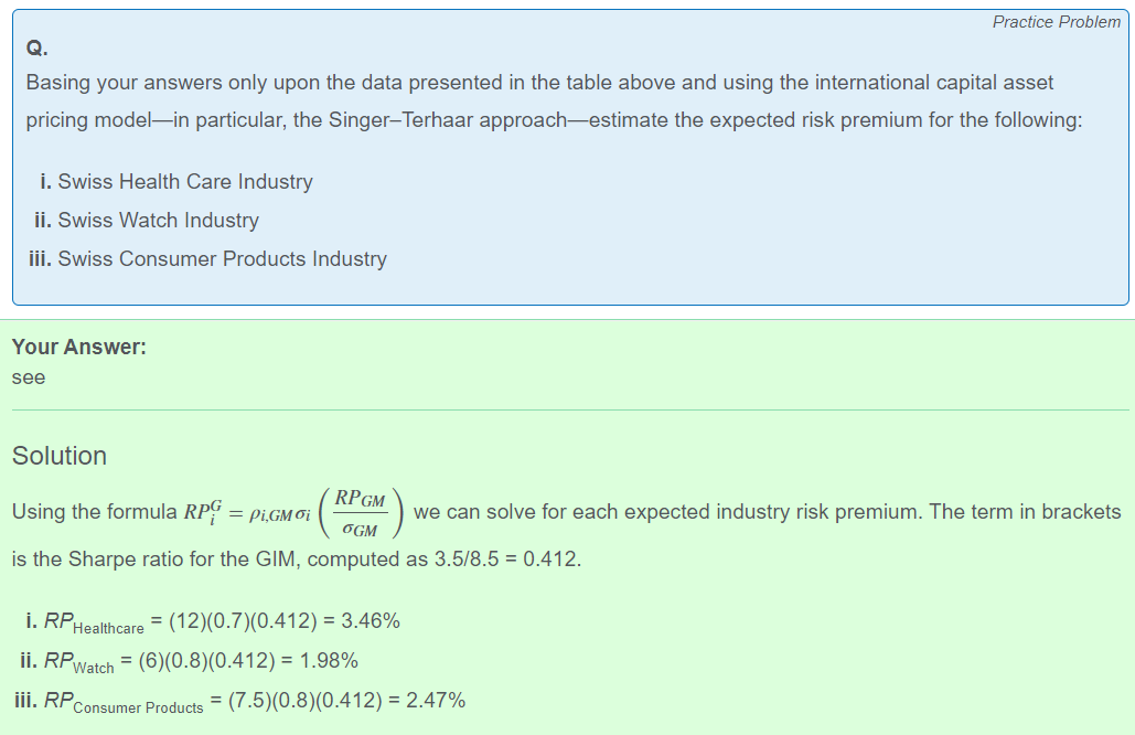
ST model (risk premium) - Demand Side (from the consumer side) Singer Terhaar Approach

CAPM -> internation CAPM

$r_i=r_f+\beta [\mathbb{E}(r_m)-r_f]$$r_i = r_f + \beta [\mathbb{E}(r_m) - r_f ]$

$r_i-r_f=RP=\beta (r_m-r_f)=\frac{co{v}_{i,m}}{{\sigma }_m^2}(r_m-r_f)$$r_i - r_f = RP = \beta (r_m - r_f) = \frac{cov_{i,m}}{\sigma^2_m}(r_m - r_f)$

$r_i-r_f={\rho }_{i,m}\frac{{\sigma }_i}{{\sigma }_m}(r_m-r_f)$$r_i - r_f = \rho_{i,m} \frac{\sigma_i}{\sigma_m}(r_m - r_f)$

$RP=r_i-r_f=\rho {\sigma }_{i}S{R}_m$$RP = r_i - r_f = \rho\ \sigma_i SR_m$ by $S{R}_m=\frac{r_m-r_f}{{\sigma }_m}$$SR _m = \frac{r_m - r_f}{\sigma_m}$

$RP=\rho {\sigma }_i\frac{RP}{{\sigma }_m}$$RP = \rho \sigma_i \frac{RP}{\sigma_m}$

• M: Global Market Portfolio (GMP)

  • $\varphi \in [0,1]$$\phi \in [0,1]$, the degree to which the asset is globally integrated. $\varphi \sim 1$$\phi \sim 1$ more integrated to the global market, $\varphi \sim 0$$\phi \sim 0$ more separate

  Steps of ST Model

  • Step 1: Fully integtated: $\varphi =1$$\phi = 1$, $R{P}_{integrated}=r_i-r_f=\rho {\sigma }_{m}S{R}_m$$RP_{integrated} = r_i - r_f = \rho\ \sigma _m SR_m$

  • Step 2: Fully Seperate: $\varphi =0$$\phi = 0$ , and because of fully seperation, asset classes are not and cannot be diversified, so $\rho =1$$\rho = 1$, so $R{P}_{seperated}=r_i-r_f={\sigma }_{m}S{R}_m$$RP_{seperated} = r_i - r_f = \sigma _m SR_m$

  • Step 3: True RP is the weighted average, $RP=\varphi R{P}_I+(1-\varphi )R{P}_S$$RP = \phi RP_{I} + (1-\phi )RP_S$

  • Step 4: $r_i=r_f+RP$$r_i = r_f + RP$

Sample Text:

• All else being equal, the Singer–Terhaar model implies that when a market becomes more globally integrated (segmented), its required return should decline (rise). As prices adjust to a lower (higher) required return, the market should deliver an even higher (lower) return than was previously expected or required by the market. Therefore, the allocation to markets that are moving toward integration should be increased. If a market is moving toward integration, its increased allocation will come at the expense of markets that are already highly integrated. This will typically entail a shift from developed markets to emerging markets.

• If hot money flows out, then CB is likely to sell foreign currency to limit domestic currency depreciation. So, CB sell foreign currency for domestic currency (卖外汇买本币，本比增加), （然后用买了的本比，买本国bond，叫 sterilise）buy domestic govenment bond (provide liquidity) => impact on both bank reserves and interest rates.

• Country B is facing the outflow of hot money, which is typically speculative capital that moves to take advantage of short-term interest rate differences between countries. When hot money flows out, the domestic currency experiences depreciation pressures. The central bank of Country B would likely sell foreign currency reserves to support the domestic currency, draining domestic liquidity in the process. To offset or "sterilize" this effect, the central bank would then buy domestic bonds, adding liquidity back into the system. This two-step process ensures that the impact of the hot money outflow on domestic interest rates and bank reserves is neutralized, making Country B the most likely to engage in this form of sterilization.

  • Step 1: Sterilise. 当 hot money 流出，相当于 资本外逃，foreign investor 卖本币买外币 撤离本国市场。CB 为了防止本币贬值，卖外币买本币。如此操作市场上 本币流动性会降低。

  • Step 2: Open Market Operation，CB 买 bond，为市场注入流动性

• the Composition of each country's currency portfolio. 外国人持有本币的形式，如果持有的 equity 那么比较好，但是 持有 domestic debt 不好，因为如果本国还不上钱，那么 主权违约。supportive of the currency: Public debt is less supportive because it has to be serviced and must be either repaid or refinanced, potentially triggering a crisis. Some types of flows and holdings are considered to be more or less supportive of the currency. Investments in private equity represent long-term capital committed to the market and are most supportive of the currency. Public equity would likely be considered the next most supportive of the currency. Debt investments are the least supportive of the currency.

Real Estate

illiquidy, heterogeneous (各个不一样), maintenance and operation cost, Appraisals

• Real Estate Cycles: high quality properties are less cyclical, low quality properties are more cyclical

DCF

In level II

$V_0=\frac{NO{I}_1}{r-g}$$V_0 = \frac{NOI_1}{r-g}$ => $r=\frac{NO{I}_1}{V_0}+g$$r = \frac{NOI_1}{V_0} + g$

We get to the formula by composing three parts

1. Cap Rate: $\frac{NO{I}_1}{V_0}$$\frac{NOI_1}{V_0}$, 经营带来的 income return, should be current cap rate

2. $g_{nominal}=g_{realNOI}+\pi$$g_{nominal} = g_{realNOI} + \pi$

3. $-\mathrm{\%}\mathrm{\Delta }CapRate$$-\%\Delta CapRate$ repricing, coz $\text{Capital Gain}=\frac{V_1-V_0}{V_0}$$\text{Capital Gain} = \frac{V_1 - V_0}{V_0}$ 但是因为 估值上升 即 V 提升带来的 Capital Gain 会使 Captial Rate 在分母的 V 变大。所以 Capital Gain & Capital Rate are negative correlated.

$r=CapRate+NOIgrowth-\mathrm{\%}\mathrm{\Delta }CapRate$$r = CapRate + NOI \ growth - \%\Delta CapRate$

Factors Affecting the Cap Rate

• Interest rate increase => NOI increase => Cap Rate increase

• vacancy rate increase => $V_0$$V_0$ decrease => Cap Rate Increase

• availability of credit and debts 信贷多，买房多demand of houses increase => $V_0$$V_0$ increase => Cap Rate decrease

Risk Premium

CF of real estate = 租金 + Cap Gain增值

$r_{house}=r_f+TP+CP+EP+LP$$r_{house} = r_f + TP + CP + EP + LP$

term premium, credit premium, equilty risk premium (cap gain), liquidity premium

REITs

短期像 equity，长期才像 real estate

• strongly correlated with equity in the short term

• only correlated with direct real estate in the long term

• REITs use significant leverage, to make it compare with direct real estate, REITs should be unlevered first

• after adjusting the leverage of REITs, it has higher return and low volatility

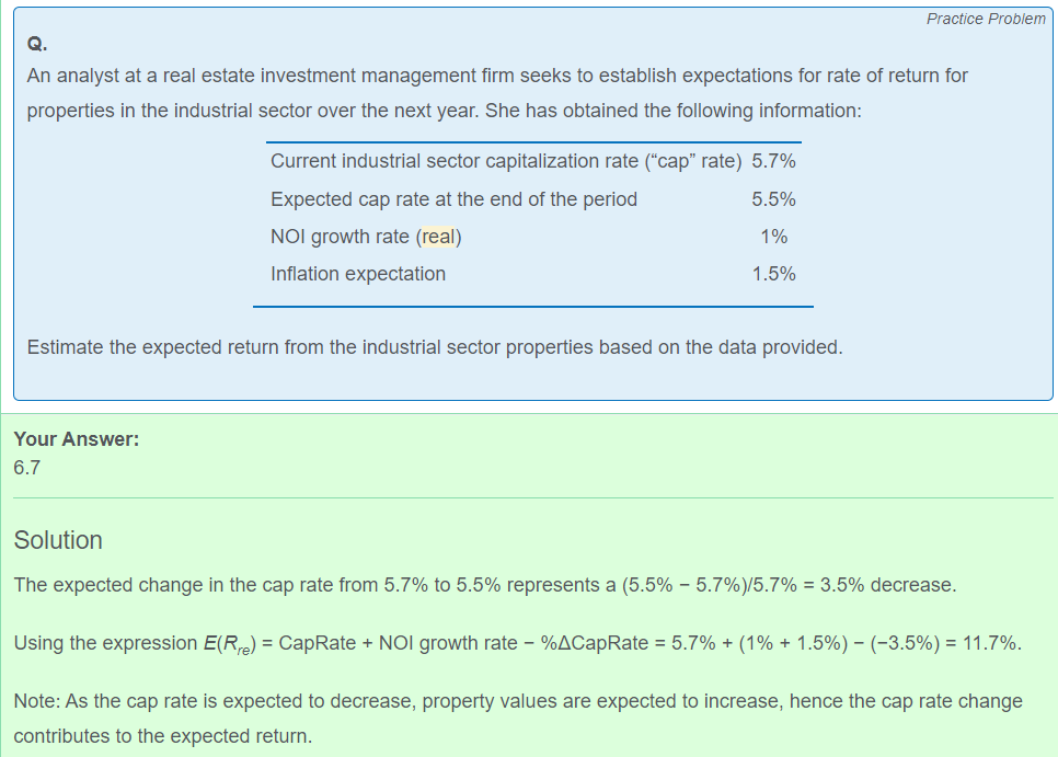
An estimate of the long-run expected or required return for commercial real estate equals the sum of the capitalisation rate (cap rate) plus the growth rate (constant) of net operating income (NOI).

$ExpectedRequiredRate=CapRate+NOI$$Expected\ Required\ Rate = Cap\ Rate+NOI$

Sample Text: An estimate of the long-run expected or required return for commercial real estate equals the sum of the capitalisation rate (cap rate) plus the growth rate (constant) of net operating income (NOI). Plus the percentage change of NOI.

Expected Required Rate: $\mathbb{E}(R_{re})=CapRate+NO{I}_{Nominal}-\mathrm{\%}\mathrm{\Delta }CapRate$$\mathbb{E}(R_{re}) = Cap\ Rate+NOI_{Nominal}-\%\Delta CapRate$

$NO{I}_{nominal}=NO{I}_{real}+Inflation$$NOI_{nominal} = NOI_{real }+ Inflation$

Exchange Rate

Current Acount: Three factors

• Trade Flows: small impacts. As trade normally has financial hedge, the effects are hedged. Large trade flows without large financing flows in foreign exchange markets likely indicates a crisis.

• PPP: less impacts in short-term. Inflation and exchange are correlated through UIP

• Current Account: large impacts. if 国内（本币）贵, import foreign, CA deficits 本币流出 未来本币贬值。vice versa.

Capital Mobility

by UIP, (e is in d/f) $e_1-e_0\approx r_d-r_f$$e_1 -e_0 \approx r_d - r_f$, and then add premiums

$E(\mathrm{\%}\mathrm{\Delta }{S}_{d/f})=(r_d-r_f)+(Ter{m}_d-Ter{m}_f)+(Credi{t}_d-Credi{t}_f)+(Equit{y}_d-Equit{y}_f)+(Liquidit{y}_d-Liquidit{y}_f)$$E(\%\Delta S_{d/f}) = (r_d -r_f) + (Term_d - Term_f) + (Credit_d - Credit_f )+ (Equity_d - Equity_f) + (Liquidity_d - Liquidity_f)$

• Overshooting

  本币过度升值。在超短期 domestic interest rate increase, => FDI increase, => FX increase more

  ?? wtb

• Hot Money

Volatility Forecasting

• Sample VCV, 用样本的资产 sampel statistics 估计 consistent and unbiased

• Factor-based VCV, 因为用 factors to estimate the variance covariance matrix, so the estimate is biased and inconsistent

• Shrinkage method <- weighted average

下为 Factor-based VCV

$r_i={\beta }_0+{\beta }_1{F}_1+{\beta }_2{F}_2+\cdots +{ϵ}_i$$r_i = \beta_0 + \beta_1 F_1 + \beta_2 F_2 + \cdots +\epsilon_i$

${\sigma }_i^2={\beta }_1^2{\sigma }_{F_1}^2+{\beta }^2{\sigma }_{F_2}^2+2{\beta }_1{\beta }_{2}co{v}_{1,2}+{\sigma }_{ϵ}^2+\cdots$$\sigma_i^2 = \beta_1^2\sigma^2_{F_1} + \beta^2\sigma^2_{F_2} + 2\beta_1\beta_2 cov_{1,2} + \sigma_{\epsilon}^2 + \cdots$

${\sigma }_i^2=\sum _{m=1}^K\sum _{n=1}^K{\beta }_{i,m}{\beta }_{m,n}co{v}_{m,n}+{\sigma }_{{ϵ}_i}^2$$\sigma_i^2 = \sum_{m=1}^K \sum_{n=1}^K \beta_{i,m}\beta_{m,n} cov_{m,n} + \sigma_{\epsilon_i}^2$

,coz

• Error terms and Factors are uncorrelated by the property of OLS

• Factors amid might be correlated, so there are covariance term between factors

Drawbacks

1. 用历史估计未来, biased

2. 如果 low liquidity 流动性差，则需要 appraisal ，那么数据要 smoothing

   result in low volatile and low correlation

   因为两组资产通常受到大的经济环境影响，价格的波动原本应趋于一致。但是现在要把这种趋于一致的波动的一方给平滑了，变成一方波动，一方不波动了，那么两者的相关性就变小了。

3. Volatility Clustering

To overcome those drawbacks, we would use those three methods.

1. Shrinkage Estimate

   • Shrinkage estimate is the combination of the sample and target (factor-based) 相当于sample 和 factor-based的加权平均

   • 但是 依然 biased

2. 防止 smoothing，

   $R_t=\lambda R_{t-1}+(1-\lambda )r_t$$R_t = \lambda R_{t-1} + (1-\lambda) r_t$

   • $R_t$$R_t$ 为市场上可见的 appraisal value

   • $r_t$$r_t$ 为真实值

     $Var(R_t)={\lambda }^{2}Var(R_{t-1})+(1-\lambda {)}^{2}Var(r_t)+2\lambda (1-\lambda )cov(R_{t-1},r_t)$$Var(R_t) = \lambda^2 Var(R_{t-1}) + (1-\lambda)^2 Var(r_t) + 2\lambda (1-\lambda)cov(R_{t-1}, r_t)$.

     As $r_t$$r_t$ and $R_{t-1}$$R_{t-1}$ are irrelevant, $cov\to 0$$cov \to 0$.

     We assume also $Var(R_t)=Var(R_{t-1})$$Var(R_t) = Var(R_{t-1})$ that we have same appraisal variance.

     Thus, $Var(r_t)=\frac{1-{\lambda }^2}{(1-\lambda {)}^2}Var(R_t)=\frac{1+\lambda }{1-\lambda }Var(R_t)$$Var(r_t) = \frac{1-\lambda^2}{(1-\lambda)^2}Var(R_t) = \frac{1+\lambda}{1-\lambda}Var(R_t)$

     • As the coefficient must be greater than 1, $Var(r_t)>Var(R_t)$$Var(r_t) > Var(R_t)$

     • The greater the $\lambda$$\lambda$, the more $Var(r_t)>>Var(R_t)$$Var(r_t) >> Var(R_t)$

     • 意味着smooth的越多，则estimate 的 var 比真实的小的越多

3. ARCH Autoregressive Condition Heteroskedasticity

   • ${\sigma }_t^2=\gamma +\alpha {\sigma }_{t-1}^2+\beta {\eta }_t^2$$\sigma^2_t = \gamma +\alpha \sigma_{t-1}^2 + \beta \eta_t^2$

     ${\eta }_t^2$$\eta_t^2$ is the unexpected component of return, resulted from the previous period's vol, ${\sigma }_{t-1}^2$$\sigma_{t-1}^2$

     ${\eta }_t^2$$\eta_t^2$ is not the error term

   • The error term should be instead, ${\eta }_t^2-{\sigma }_{t-1}^2$$\eta_t^2 - \sigma_{t-1}^2$, which is the eta less the vol from previous period.

   • Then, we reform the formula

     ${\sigma }_t^2=\gamma +\alpha {\sigma }_{t-1}^2+\beta ({\eta }_t^2-{\sigma }_{t-1}^2)+\beta {\sigma }_{t-1}^2$$\sigma_t^2 = \gamma + \alpha \sigma_{t-1}^2 + \beta (\eta_t^2 - \sigma_{t-1}^2) + \beta \sigma_{t-1}^2$

     ${\sigma }_t^2=\gamma +(\alpha +\beta ){\sigma }_{t-1}^2+\beta ({\eta }_t^2-{\sigma }_{t-1}^2)$$\sigma_t^2 = \gamma + (\alpha +\beta )\sigma_{t-1}^2 + \beta (\eta_t^2 - \sigma_{t-1}^2)$

     • If $\beta =0$$\beta=0$, then no shocks, then variance is deterministic

     • Take expectation from both sides,

       $\mathbb{E}({\sigma }_t^2)=\mathbb{E}(\gamma )+\mathbb{E}((\alpha +\beta ){\sigma }_{t-1}^2)+\mathbb{E}(\beta ({\eta }_t^2-{\sigma }_{t-1}^2))$$\mathbb{E}( \sigma_t^2 )=\mathbb{E}( \gamma )+ \mathbb{E}((\alpha +\beta )\sigma_{t-1}^2) + \mathbb{E}(\beta (\eta_t^2 - \sigma_{t-1}^2) )$

       the expectation of the error term is zero, and assume $\mathbb{E}({\sigma }_t^2)=\mathbb{E}({\sigma }_{t-1}^2)$$\mathbb{E}(\sigma_{t}^2) =\mathbb{E}(\sigma_{t-1}^2)$ over time, then

       $\mathbb{E}({\sigma }_t^2)=\gamma +(\alpha +\beta )\mathbb{E}({\sigma }_t^2)$$\mathbb{E}( \sigma_t^2 )= \gamma + (\alpha +\beta )\mathbb{E}(\sigma_{t}^2)$

       $\mathbb{E}({\sigma }_t^2)=\frac{\gamma }{1-\alpha -\beta }$$\mathbb{E}(\sigma_t^2) = \frac{\gamma}{1-\alpha - \beta}$

       We need $1-\alpha +\beta >1$$1 - \alpha + \beta >1$ to make the expectation of var is positive over time