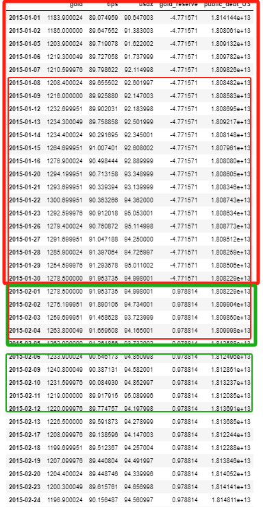
Use the panel data of the red block to predict the mean of green block. Then, roll it.
import numpy as np
import pandas as pd
import statsmodels.api as sm
import matplotlib.pyplot as plt

import yfinance as yf
import requests

import cufflinks as cf; cf.go_offline()
plt.style.use('fivethirtyeight')
# Define the start and end dates for the data
start_date = '2010-01-01'

# # Retrieve the data
# # Gold Price
data_gold = yf.download('GC=F', start=start_date)
# # TIPS
data_tips = yf.download('TIP', start=start_date)
# # USDollar Index
data_usdindex = yf.download('DX=F', start=start_date)

price_gold = data_gold['Adj Close'].rename('gold')
price_tips = data_tips['Adj Close'].rename('tips')
price_usdindex = data_usdindex['Adj Close'].rename('usdx')
df = pd.concat([price_gold, price_tips, price_usdindex],axis=1)
df_diff = df.diff()

df.to_csv(r'./Data/data_from_yfinance.csv')
[*********************100%%**********************]  1 of 1 completed
[*********************100%%**********************]  1 of 1 completed
[*********************100%%**********************]  1 of 1 completed
start_date = '2010-01-01'

df_from_yf = pd.read_csv(r'./Data/data_from_yfinance.csv', index_col='Date', parse_dates=True)
df_from_yf
| gold | tips | usdx | |
|---|---|---|---|
| Date | |||
| 2010-01-04 | 1117.699951 | 73.639183 | 77.830002 |
| 2010-01-05 | 1118.099976 | 73.879532 | 77.849998 |
| 2010-01-06 | 1135.900024 | 73.688652 | 77.654999 |
| 2010-01-07 | 1133.099976 | 73.801781 | 78.105003 |
| 2010-01-08 | 1138.199951 | 73.957268 | 77.654999 |
| ... | ... | ... | ... |
| 2024-04-16 | 2390.800049 | 105.349998 | 106.065002 |
| 2024-04-17 | 2371.699951 | 105.760002 | 105.764000 |
| 2024-04-18 | 2382.300049 | 105.620003 | 105.982002 |
| 2024-04-19 | 2398.399902 | 105.779999 | 105.984001 |
| 2024-04-22 | 2382.699951 | NaN | 105.885002 |
3600 rows × 3 columns
df_from_yf.iplot(y='gold', secondary_y = [ 'tips', 'usdx'])
df_from_yf.corr()
| gold | tips | usdx | |
|---|---|---|---|
| gold | 1.000000 | 0.734716 | 0.240488 |
| tips | 0.734716 | 1.000000 | 0.616567 |
| usdx | 0.240488 | 0.616567 | 1.000000 |
df_from_yf[df_from_yf.index>'2020'].corr()
| gold | tips | usdx | |
|---|---|---|---|
| gold | 1.000000 | 0.072961 | 0.102308 |
| tips | 0.072961 | 1.000000 | -0.609331 |
| usdx | 0.102308 | -0.609331 | 1.000000 |
df_from_yf[df_from_yf.index > '2020'].iplot(y='gold', secondary_y = [ 'tips', 'usdx'])
df_from_yf[df_from_yf.index>'2023'].corr()
| gold | tips | usdx | |
|---|---|---|---|
| gold | 1.000000 | 0.516854 | 0.000794 |
| tips | 0.516854 | 1.000000 | -0.676702 |
| usdx | 0.000794 | -0.676702 | 1.000000 |
df_from_yf[df_from_yf.index > '2023'].iplot(y='gold', secondary_y = [ 'tips', 'usdx'])
Periodically download from the website
https://www.gold.org/goldhub/data/gold-reserves-by-country
2024April: https://www.gold.org/download/file/7741/1
start_date = '2015-01-01'
df_reserve_change = pd.read_excel(r'./Data/Changes_latest_as_of_Apr2024_IFS.xlsx', sheet_name='Monthly',skiprows=7, parse_dates=True, index_col='Country')
df_reserve_change = df_reserve_change.T.iloc[2:,]
df_reserve_change.index = pd.to_datetime(df_reserve_change.index)
df_reserve_change = df_reserve_change[df_reserve_change.index >= start_date]
df_reserve_change.cumsum()[df_reserve_change.sum().sort_values()[-10:].index].iplot()
df_gold_reserve = df_reserve_change.sum(axis=1).cumsum()
df_gold_reserve.name = 'gold_reserve'
df_gold_reserve.iplot()
https://fiscaldata.treasury.gov/datasets/debt-to-the-penny/debt-to-the-penny
# Define the API endpoint URL
base_url = "https://api.fiscaldata.treasury.gov/services/api/fiscal_service/"
endpoint = "v2/accounting/od/debt_to_penny"
Num_Days = 252 * 10
parameters = f'?sort=-record_date&page[number]=1&page[size]={Num_Days}'
full_url = base_url + endpoint + parameters

# Make a GET request to the API
response = requests.get(full_url)

# Check if the request was successful (status code 200)
if response.status_code == 200:
    # Parse the JSON response
    data = response.json()
    dict_debt = {}
    # Access the data from the response
    for entry in data["data"]:
#         print(f"Record Date: {entry['record_date']}, Debt to Penny: {entry['tot_pub_debt_out_amt']}")
        dict_debt[entry['record_date']] = entry['tot_pub_debt_out_amt']
else:
    print(f"Failed to retrieve data. Status code: {response.status_code}")
df_publicDebtUS = pd.Series(dict_debt, name = 'public_debt_US')
df_publicDebtUS = df_publicDebtUS.astype('f')
df_publicDebtUS.index = pd.to_datetime(df_publicDebtUS.index)

df_publicDebtUS.sort_index().iplot()
df = pd.concat([df_from_yf, df_gold_reserve, df_publicDebtUS],axis=1)
df = df.fillna(method='ffill') # front fill all NAN with previously available figure
df = df.dropna()
# df = df[df.index > '2020']

# Save DataSet
df.to_csv(r'./Data/DataSet.csv')
def run_regression(df, robust = False, constant = True):
    """
    the first column is the Y
    the rest are X
    """
    # Split the DataFrame into the dependent variable (Y) and independent variables (X)
    Y = df.iloc[:, 0]  # First column
    X = df.iloc[:, 1:]  # Remaining columns

    # Add a constant to the independent variables (intercept)
    X = sm.add_constant(X)

    if not robust: # if robust is switched off
        # Fit the regression model
        model = sm.OLS(Y, X).fit()
    else:
        # fit the model with robust s.e.
        model = sm.OLS(Y, X).fit(cov_type='HC3')  # Use HC3 for robust standard errors

    # Print the model summary
    print(model.summary())
    return model


model = run_regression(df)
                            OLS Regression Results
==============================================================================
Dep. Variable:                   gold   R-squared:                       0.932
Model:                            OLS   Adj. R-squared:                  0.932
Method:                 Least Squares   F-statistic:                 1.095e+04
Date:                Mon, 22 Apr 2024   Prob (F-statistic):               0.00
Time:                        13:18:56   Log-Likelihood:                -13938.
No. Observations:                2393   AIC:                         2.788e+04
Df Residuals:                    2389   BIC:                         2.791e+04
Df Model:                           3
Covariance Type:            nonrobust
==================================================================================
                     coef    std err          t      P>|t|      [0.025      0.975]
----------------------------------------------------------------------------------
const              0.0095      0.001      7.293      0.000       0.007       0.012
tips               9.4253      0.242     38.957      0.000       8.951       9.900
usdx              -6.5777      0.245    -26.874      0.000      -7.058      -6.098
gold_reserve      -0.0240      0.005     -4.967      0.000      -0.033      -0.014
public_debt_US  5.247e-11   1.29e-12     40.795      0.000    4.99e-11     5.5e-11
==============================================================================
Omnibus:                      195.470   Durbin-Watson:                   0.026
Prob(Omnibus):                  0.000   Jarque-Bera (JB):              299.057
Skew:                           0.629   Prob(JB):                     1.15e-65
Kurtosis:                       4.190   Cond. No.                     1.07e+15
==============================================================================

Notes:
[1] Standard Errors assume that the covariance matrix of the errors is correctly specified.
[2] The condition number is large, 1.07e+15. This might indicate that there are
strong multicollinearity or other numerical problems.
if seperate with the train and test sets
def plot_predict_model(df_full, loc_train = 0.8, loc_test = 0.2):
    # seperate the train / test set
    set_train = df[:int(len(df)*loc_train)]
    set_test = df[int(len(df)*(1-loc_test)):]

    # train the model using the train set
    temp_model = run_regression(set_train)

    # predict and plot
    y_predicted = set_test.iloc[:,1:].shift(1) @ temp_model.params[1:] + temp_model.params[0] # use past 1 day data to estimate the next day
    y_predicted.name = 'predicted'
    y_real = set_test.iloc[:,0]
    results = pd.concat([y_predicted, y_real], axis=1).iplot()

    return results
results = plot_predict_model(df, loc_train=1)
                            OLS Regression Results
==============================================================================
Dep. Variable:                   gold   R-squared:                       0.932
Model:                            OLS   Adj. R-squared:                  0.932
Method:                 Least Squares   F-statistic:                 1.095e+04
Date:                Mon, 22 Apr 2024   Prob (F-statistic):               0.00
Time:                        13:18:56   Log-Likelihood:                -13938.
No. Observations:                2393   AIC:                         2.788e+04
Df Residuals:                    2389   BIC:                         2.791e+04
Df Model:                           3
Covariance Type:            nonrobust
==================================================================================
                     coef    std err          t      P>|t|      [0.025      0.975]
----------------------------------------------------------------------------------
const              0.0095      0.001      7.293      0.000       0.007       0.012
tips               9.4253      0.242     38.957      0.000       8.951       9.900
usdx              -6.5777      0.245    -26.874      0.000      -7.058      -6.098
gold_reserve      -0.0240      0.005     -4.967      0.000      -0.033      -0.014
public_debt_US  5.247e-11   1.29e-12     40.795      0.000    4.99e-11     5.5e-11
==============================================================================
Omnibus:                      195.470   Durbin-Watson:                   0.026
Prob(Omnibus):                  0.000   Jarque-Bera (JB):              299.057
Skew:                           0.629   Prob(JB):                     1.15e-65
Kurtosis:                       4.190   Cond. No.                     1.07e+15
==============================================================================

Notes:
[1] Standard Errors assume that the covariance matrix of the errors is correctly specified.
[2] The condition number is large, 1.07e+15. This might indicate that there are
strong multicollinearity or other numerical problems.
VIX also shows statistically significant
# # USDollar Index
data_vix = yf.download('^VIX', start=start_date)

price_vix = data_vix['Adj Close'].rename('vix')
df_temp = pd.concat([df, price_vix], axis =1).dropna()
[*********************100%%**********************] 1 of 1 completed
model_temp = run_regression(df_temp)
                            OLS Regression Results
==============================================================================
Dep. Variable:                   gold   R-squared:                       0.934
Model:                            OLS   Adj. R-squared:                  0.934
Method:                 Least Squares   F-statistic:                     8328.
Date:                Mon, 22 Apr 2024   Prob (F-statistic):               0.00
Time:                        13:18:57   Log-Likelihood:                -13585.
No. Observations:                2340   AIC:                         2.718e+04
Df Residuals:                    2335   BIC:                         2.721e+04
Df Model:                           4
Covariance Type:            nonrobust
==================================================================================
                     coef    std err          t      P>|t|      [0.025      0.975]
----------------------------------------------------------------------------------
const              0.0057      0.001      3.896      0.000       0.003       0.009
tips               8.9515      0.248     36.114      0.000       8.465       9.438
usdx              -6.7403      0.244    -27.629      0.000      -7.219      -6.262
gold_reserve      -0.0326      0.005     -6.622      0.000      -0.042      -0.023
public_debt_US  5.437e-11   1.31e-12     41.611      0.000    5.18e-11    5.69e-11
vix                1.9966      0.244      8.193      0.000       1.519       2.475
==============================================================================
Omnibus:                      160.805   Durbin-Watson:                   0.029
Prob(Omnibus):                  0.000   Jarque-Bera (JB):              251.765
Skew:                           0.543   Prob(JB):                     2.14e-55
Kurtosis:                       4.185   Cond. No.                     1.10e+15
==============================================================================

Notes:
[1] Standard Errors assume that the covariance matrix of the errors is correctly specified.
[2] The condition number is large, 1.1e+15. This might indicate that there are
strong multicollinearity or other numerical problems.
results = plot_predict_model(df_temp, loc_train = 1)
                            OLS Regression Results
==============================================================================
Dep. Variable:                   gold   R-squared:                       0.932
Model:                            OLS   Adj. R-squared:                  0.932
Method:                 Least Squares   F-statistic:                 1.095e+04
Date:                Mon, 22 Apr 2024   Prob (F-statistic):               0.00
Time:                        13:18:57   Log-Likelihood:                -13938.
No. Observations:                2393   AIC:                         2.788e+04
Df Residuals:                    2389   BIC:                         2.791e+04
Df Model:                           3
Covariance Type:            nonrobust
==================================================================================
                     coef    std err          t      P>|t|      [0.025      0.975]
----------------------------------------------------------------------------------
const              0.0095      0.001      7.293      0.000       0.007       0.012
tips               9.4253      0.242     38.957      0.000       8.951       9.900
usdx              -6.5777      0.245    -26.874      0.000      -7.058      -6.098
gold_reserve      -0.0240      0.005     -4.967      0.000      -0.033      -0.014
public_debt_US  5.247e-11   1.29e-12     40.795      0.000    4.99e-11     5.5e-11
==============================================================================
Omnibus:                      195.470   Durbin-Watson:                   0.026
Prob(Omnibus):                  0.000   Jarque-Bera (JB):              299.057
Skew:                           0.629   Prob(JB):                     1.15e-65
Kurtosis:                       4.190   Cond. No.                     1.07e+15
==============================================================================

Notes:
[1] Standard Errors assume that the covariance matrix of the errors is correctly specified.
[2] The condition number is large, 1.07e+15. This might indicate that there are
strong multicollinearity or other numerical problems.
That Preidiction is counter intuitive, as the simply model might hardly perform better than Deep Learning model in prediction.
Let's see how a LSTM works then.
SPLIT_RATE = 0.80
SPLIT = int(len(df) * SPLIT_RATE)
df_train = df.iloc[:SPLIT,]
df_test = df.iloc[SPLIT:,]

df_train_X = df_train.copy()
df_train_y = df_train.iloc[:,0]
df_train_X
| gold | tips | usdx | gold_reserve | public_debt_US | |
|---|---|---|---|---|---|
| 2015-01-01 | 1183.900024 | 89.074951 | 90.647003 | -4.771571 | 1.814144e+13 |
| 2015-01-02 | 1186.000000 | 89.647568 | 91.383003 | -4.771571 | 1.808061e+13 |
| 2015-01-05 | 1203.900024 | 89.719139 | 91.622002 | -4.771571 | 1.809132e+13 |
| 2015-01-06 | 1219.300049 | 89.727066 | 91.737999 | -4.771571 | 1.809782e+13 |
| 2015-01-07 | 1210.599976 | 89.798637 | 92.114998 | -4.771571 | 1.809826e+13 |
| ... | ... | ... | ... | ... | ... |
| 2022-06-01 | 1843.300049 | 110.265816 | 102.528999 | 3578.961501 | 3.044098e+13 |
| 2022-06-02 | 1866.500000 | 110.774353 | 101.832001 | 3578.961501 | 3.042566e+13 |
| 2022-06-03 | 1845.400024 | 111.414734 | 102.160004 | 3578.961501 | 3.041255e+13 |
| 2022-06-06 | 1839.199951 | 110.689590 | 102.446999 | 3578.961501 | 3.042089e+13 |
| 2022-06-07 | 1847.500000 | 110.953270 | 102.324997 | 3578.961501 | 3.041759e+13 |
1914 rows × 5 columns
from sklearn.preprocessing import StandardScaler
standerdiser_X = StandardScaler()
standerdiser_y = StandardScaler()
df_train_scaled_X = standerdiser_X.fit_transform(df_train_X)
df_train_scaled_y = standerdiser_y.fit_transform(df_train_y.to_numpy().reshape(-1,1))
Use the panel data of the red block to predict the mean of green block. Then, roll it.
duration = 21 # 21 workings days means 1 month
num_records = len(df_train)
window = 5
X_train = []
y_train = []

for i in range(duration, num_records, window):
    X_train.append(df_train_scaled_X[i - duration:i]) # use past 21-day data, rolling-(ly)
    y_train.append(df_train_scaled_y[i:i + window].mean()) # to estimate the future 5-day means
X_train, y_train = np.array(X_train), np.array(y_train)
from keras.models import Sequential
from keras.layers import Dense, LSTM, Dropout
model = Sequential()
model.add(LSTM(units = 50, return_sequences=True))
model.add(Dropout(0.2))
model.add(LSTM(units=50))
model.add(Dropout(0.1))
model.add(Dense(1))
model.compile(optimizer='adam', loss = 'mean_squared_error')
model.fit(X_train, y_train, epochs = 100, batch_size = 64, verbose=2)
Epoch 1/100
6/6 - 3s - 559ms/step - loss: 0.3978
Epoch 2/100
6/6 - 0s - 18ms/step - loss: 0.1049
Epoch 3/100
6/6 - 0s - 16ms/step - loss: 0.0653
Epoch 4/100
6/6 - 0s - 17ms/step - loss: 0.0574
Epoch 5/100
6/6 - 0s - 17ms/step - loss: 0.0495
Epoch 6/100
6/6 - 0s - 17ms/step - loss: 0.0407
Epoch 7/100
6/6 - 0s - 14ms/step - loss: 0.0340
Epoch 8/100
6/6 - 0s - 17ms/step - loss: 0.0337
Epoch 9/100
6/6 - 0s - 17ms/step - loss: 0.0284
Epoch 10/100
6/6 - 0s - 19ms/step - loss: 0.0293
Epoch 11/100
6/6 - 0s - 17ms/step - loss: 0.0254
Epoch 12/100
6/6 - 0s - 16ms/step - loss: 0.0269
Epoch 13/100
6/6 - 0s - 19ms/step - loss: 0.0223
Epoch 14/100
6/6 - 0s - 17ms/step - loss: 0.0256
Epoch 15/100
6/6 - 0s - 17ms/step - loss: 0.0208
Epoch 16/100
6/6 - 0s - 19ms/step - loss: 0.0215
Epoch 17/100
6/6 - 0s - 17ms/step - loss: 0.0214
Epoch 18/100
6/6 - 0s - 20ms/step - loss: 0.0203
Epoch 19/100
6/6 - 0s - 16ms/step - loss: 0.0193
Epoch 20/100
6/6 - 0s - 17ms/step - loss: 0.0191
Epoch 21/100
6/6 - 0s - 17ms/step - loss: 0.0189
Epoch 22/100
6/6 - 0s - 16ms/step - loss: 0.0216
Epoch 23/100
6/6 - 0s - 17ms/step - loss: 0.0200
Epoch 24/100
6/6 - 0s - 17ms/step - loss: 0.0208
Epoch 25/100
6/6 - 0s - 17ms/step - loss: 0.0191
Epoch 26/100
6/6 - 0s - 17ms/step - loss: 0.0192
Epoch 27/100
6/6 - 0s - 17ms/step - loss: 0.0173
Epoch 28/100
6/6 - 0s - 17ms/step - loss: 0.0184
Epoch 29/100
6/6 - 0s - 15ms/step - loss: 0.0214
Epoch 30/100
6/6 - 0s - 17ms/step - loss: 0.0181
Epoch 31/100
6/6 - 0s - 16ms/step - loss: 0.0174
Epoch 32/100
6/6 - 0s - 17ms/step - loss: 0.0187
Epoch 33/100
6/6 - 0s - 20ms/step - loss: 0.0197
Epoch 34/100
6/6 - 0s - 16ms/step - loss: 0.0186
Epoch 35/100
6/6 - 0s - 16ms/step - loss: 0.0175
Epoch 36/100
6/6 - 0s - 16ms/step - loss: 0.0176
Epoch 37/100
6/6 - 0s - 19ms/step - loss: 0.0183
Epoch 38/100
6/6 - 0s - 17ms/step - loss: 0.0189
Epoch 39/100
6/6 - 0s - 19ms/step - loss: 0.0168
Epoch 40/100
6/6 - 0s - 16ms/step - loss: 0.0190
Epoch 41/100
6/6 - 0s - 19ms/step - loss: 0.0171
Epoch 42/100
6/6 - 0s - 17ms/step - loss: 0.0166
Epoch 43/100
6/6 - 0s - 17ms/step - loss: 0.0164
Epoch 44/100
6/6 - 0s - 16ms/step - loss: 0.0150
Epoch 45/100
6/6 - 0s - 18ms/step - loss: 0.0160
Epoch 46/100
6/6 - 0s - 16ms/step - loss: 0.0150
Epoch 47/100
6/6 - 0s - 15ms/step - loss: 0.0163
Epoch 48/100
6/6 - 0s - 17ms/step - loss: 0.0194
Epoch 49/100
6/6 - 0s - 17ms/step - loss: 0.0178
Epoch 50/100
6/6 - 0s - 17ms/step - loss: 0.0161
Epoch 51/100
6/6 - 0s - 16ms/step - loss: 0.0155
Epoch 52/100
6/6 - 0s - 19ms/step - loss: 0.0158
Epoch 53/100
6/6 - 0s - 17ms/step - loss: 0.0161
Epoch 54/100
6/6 - 0s - 17ms/step - loss: 0.0170
Epoch 55/100
6/6 - 0s - 17ms/step - loss: 0.0155
Epoch 56/100
6/6 - 0s - 16ms/step - loss: 0.0135
Epoch 57/100
6/6 - 0s - 17ms/step - loss: 0.0142
Epoch 58/100
6/6 - 0s - 17ms/step - loss: 0.0156
Epoch 59/100
6/6 - 0s - 18ms/step - loss: 0.0151
Epoch 60/100
6/6 - 0s - 18ms/step - loss: 0.0158
Epoch 61/100
6/6 - 0s - 14ms/step - loss: 0.0154
Epoch 62/100
6/6 - 0s - 14ms/step - loss: 0.0143
Epoch 63/100
6/6 - 0s - 18ms/step - loss: 0.0154
Epoch 64/100
6/6 - 0s - 18ms/step - loss: 0.0172
Epoch 65/100
6/6 - 0s - 18ms/step - loss: 0.0143
Epoch 66/100
6/6 - 0s - 16ms/step - loss: 0.0166
Epoch 67/100
6/6 - 0s - 16ms/step - loss: 0.0174
Epoch 68/100
6/6 - 0s - 16ms/step - loss: 0.0142
Epoch 69/100
6/6 - 0s - 17ms/step - loss: 0.0157
Epoch 70/100
6/6 - 0s - 17ms/step - loss: 0.0145
Epoch 71/100
6/6 - 0s - 17ms/step - loss: 0.0144
Epoch 72/100
6/6 - 0s - 19ms/step - loss: 0.0142
Epoch 73/100
6/6 - 0s - 20ms/step - loss: 0.0144
Epoch 74/100
6/6 - 0s - 16ms/step - loss: 0.0143
Epoch 75/100
6/6 - 0s - 17ms/step - loss: 0.0139
Epoch 76/100
6/6 - 0s - 17ms/step - loss: 0.0141
Epoch 77/100
6/6 - 0s - 17ms/step - loss: 0.0142
Epoch 78/100
6/6 - 0s - 19ms/step - loss: 0.0144
Epoch 79/100
6/6 - 0s - 17ms/step - loss: 0.0128
Epoch 80/100
6/6 - 0s - 17ms/step - loss: 0.0143
Epoch 81/100
6/6 - 0s - 17ms/step - loss: 0.0132
Epoch 82/100
6/6 - 0s - 19ms/step - loss: 0.0140
Epoch 83/100
6/6 - 0s - 17ms/step - loss: 0.0137
Epoch 84/100
6/6 - 0s - 17ms/step - loss: 0.0125
Epoch 85/100
6/6 - 0s - 18ms/step - loss: 0.0147
Epoch 86/100
6/6 - 0s - 17ms/step - loss: 0.0139
Epoch 87/100
6/6 - 0s - 17ms/step - loss: 0.0144
Epoch 88/100
6/6 - 0s - 20ms/step - loss: 0.0130
Epoch 89/100
6/6 - 0s - 16ms/step - loss: 0.0151
Epoch 90/100
6/6 - 0s - 17ms/step - loss: 0.0140
Epoch 91/100
6/6 - 0s - 17ms/step - loss: 0.0157
Epoch 92/100
6/6 - 0s - 17ms/step - loss: 0.0168
Epoch 93/100
6/6 - 0s - 17ms/step - loss: 0.0153
Epoch 94/100
6/6 - 0s - 17ms/step - loss: 0.0137
Epoch 95/100
6/6 - 0s - 17ms/step - loss: 0.0147
Epoch 96/100
6/6 - 0s - 17ms/step - loss: 0.0139
Epoch 97/100
6/6 - 0s - 16ms/step - loss: 0.0133
Epoch 98/100
6/6 - 0s - 17ms/step - loss: 0.0131
Epoch 99/100
6/6 - 0s - 17ms/step - loss: 0.0118
Epoch 100/100
6/6 - 0s - 18ms/step - loss: 0.0130
<keras.src.callbacks.history.History at 0x1deb8a48990>
df_test_standardised = standerdiser_X.transform(df_test)
df_test_standardised.shape
(479, 5)
duration = 21
num_records_test = len(df_test_standardised)
window = 5

df_test_predict = []
y_true = []
list_index = []
for i in range(duration, num_records_test, window):
    df_test_predict.append(df_test_standardised[i-duration:i])
    y_true.append(df_test[i : i + window]['gold'].mean())
    list_index.append(df_test.index[i])
df_test_predict, y_true = np.array(df_test_predict), np.array(y_true)
print(df_test_predict.shape)
print(y_true.shape)
(92, 21, 5)
(92,)
y_predicted = model.predict(df_test_predict)
3/3 ━━━━━━━━━━━━━━━━━━━━ 1s 184ms/step
y_predicted_result = standerdiser_y.inverse_transform(y_predicted)
y_predicted_result.shape
(92, 1)
table_result = pd.DataFrame([y_true, y_predicted_result.reshape(1,-1)[0]], columns=list_index).T
table_result = table_result.rename(columns={0:'TrueValue',1:'Predicted'})
table_result.iplot()