The first approach is that analysts focus on flows of export and imports to establish what the net trade flows are and how large they are relative to the economy and other, potentially larger financing and investment flows. The approach also considers differences between domestic and foreign inflation rates that relate to the concept of purchasing power parity. Under PPP, the expected percentage change in the exchange rate should equal the difference between inflation rates. The approach also considers the sustainability of current account imbalances, reflecting the difference between national saving and investment.
The second approach is that the analysis focuses on capital flows and the degree of capital mobility. It assumes that capital seeks the highest risk-adjusted return. The expected changes in the exchange rate will reflect the differences in the respective countries’ assets’ characteristics such as relative short-term interest rates, term, credit, equity and liquidity premiums. The approach also considers hot money flows and the fact that exchange rates provide an across the board mechanism for adjusting the relative sizes of each country’s portfolio of assets.
Developed by John B. Taylor – aims to be a rule of thumb
If the Federal Reserve decides to increase the liquidity, it would then buy bonds and put more money into the market. As there is more money to lend, the interest rate would go down.
The monetary policy aims to target the inflation rate. Considering the Philips curve, there is a trade-off between unemployment and inflation. Unemployment could be replaced by its counterpart, economic growth. We consider the goal of the monetary department to balance GDP and Inflation.
The Fed normally has a target interest rate, the federal funds rate, which is the overnight rate in the interbank market for short term lending. How should the monetary policy set the target interest rate? This is the key discussion of the Taylor rule.
$$i=i^*+a (\pi – \pi^*) – b(U-U^*)$$
By the Philips curve, we replace unemployment with output. As we separate the interest rate to be the real interest rate and the inflation rate.
The output gap could be considered to be by what percentage of the current GDP is below the Potential GDP.
Clearly, the Taylor rule is intuitively to be correct.
If there is an inflation gap the current inflation is greater than the target, which also means there is an extra money supply moving the CPI upward, then the Fed should conduct a contractionary monetary policy, and it should set a higher interest rate.
If the GDP growth is lower than the target (potential), or if the unemployment rate is greater than the target, then the Fed would like to stimulate the market. Thus, it would decrease the interest rate.
For the Taylor rule, John Taylor did not mean the monetary policy should follow it. It is not a law but just a rule of thumb. Normally, we also set the coefficients \(a\) and \(b\) to be 1\2. However, if we think the government would pay more attention to the inflation target, then we could certainly increase the weight of inflation gap.
The “unpleasant arithmetic” stated that if the government has leadership, it can coerce expansions in money.
In contrast, FTPL says that the above restrictions are not a constraint to the CB or government. Instead, it is an equilibrium relation.
As a consequence, the CB and the government may choose policies independent of the above constraint. In the end, the price level \(p_t\) must then adjust such that the equation holds.
Here, I would apply the equation of exchange and government budget constraint to explain how inflation is generated by government deficits. Recalling the government budget constraint,
By denoting real government debt as \( \hat{d}_t=\frac{d_t}{p_{t-1}}\), and replace \( (1+r_t)=(1+i_t)\frac{P_{t-1}}{P_t}=\frac{1+i_t}{1+\pi_t} \) and \( m_t = p_t y_t \), then we get all variables are in real terms,
At the steady state \( g_t=g_{t+1}=g, \tau_t=\tau_{t+1}=\tau \) and so on, and thus,
$$ \underbrace{g+r\hat{d}-\tau }_{Growth\ of \ interest\ deficits}= \underbrace{\frac{p_t-p_{t-1}}{p_t}}_{Seignorage} \times y$$
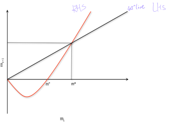
From the above equation, we can find that if inflation increases then it means the RHS increases. The LHS consists of two parts. Government Spendings \( g + r\hat{d}\) and government revenues \( \tau \). That means the government is getting deficits if the LHS rises. Meanwhile, the RHS increases and so inflation grows.
In sum, we find that government deficits, in the long run, would induce inflation. The zero-inflation condition is to make the LHS of the equation equal to zero (government spendings offset government revenue).
Now assume that money supply follows \(M_{t+1}=(1+\mu)M_t\). Also assume government spending is zero, so all seignorage is redistributed as a (negative) lum-sum tax. ENdowments are constant and given by \(y\).
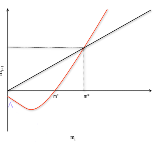
If \( \lim_{m\rightarrow 0}v'(m)m=0\), then \(m^*=0\) is also a steady state equilibrium.
P.S. \(u'(y)=v'(m”)\)
In addition, there exists an \(m”>0\) such that
$$ u'(y)=v'(m”) $$
which implies that \(m_{t+1}\leq0\) for \(m_t\leq m”\).
The relationship could be expressed by the figure below.
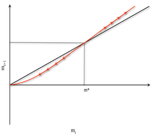
If the initial condition of \(m_t\) is at the right of \(m^*\), then RHS is always greater than the LHS and would result in \(\lim_{t \rightarrow \infty} m_t \rightarrow \infty\). No steady state and violate the transversality condition. Thus, \(m_0\) cannot be at the right of \(m^*\).
If the \(m_0\) at the left of \(m^*\), then \(m_t\) would converge to 0 (as the similar logic above). Therefore, as \(m_t \rightarrow 0\), \(p_t\ rightarrow \infty\) even if \(M_t\) keeps constant. That would lead to hyperinflation.
In that scenario, the unique equilibrium is \(m_t=m^*>0\), the price level is determined. Prices, in this case, must be growing at precisely the same rates as money, which adhere to the monetarist doctrine. However, the economy can also display speculative hyperinflation in which inflation far outpace money growth.
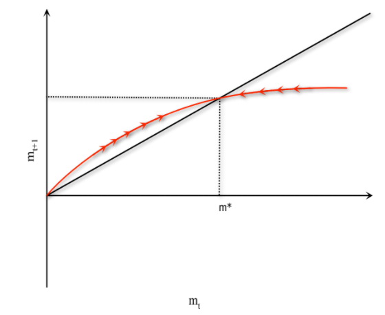
In addition, different forms of the RHS might lead to different results.
E.G. the concavity of RHS, the interaction point at zero, etc would all affect the equilibrium condition.
Fiscal Policy also helps to get out of the liquidity trap.
Ricardian Equivalence in the Cash-in-Advance Model
Ricardian Equivalence states that the government finance the government spending, \(g_t\), by debts or taxes is irrelevant.
Consider tax, \(T_t\), as government steals money from the private sectors. Then, borrowing money is the same, because the government needs to finance the repayments by taxes as well. Government repay with one hand and steal (or tax) the same amount with the other hand. Thus, funds lent out to the government will never be given back.
Therefore, borrowing is the same as tax. However, this is not true sometimes, because debts and interest can help smooth consumption.
The Ricardian equivalence cannot be shown in the Cash-in-Advance model because tax and debts won’t be shown in the Euler equation, once markets clear and model achieves the equilibrium.
and \( x_{t+1}\geq0, i_{t+1}\geq0, x_{t+1}\times i_{t+1}=0\). Clearly, no taxes and debts appear in the equations ( as tax and debts are represented by the government spending).
A interesting phenomena appears that \(\uparrow g \Rightarrow \uparrow\hat{y}\). Also, government spending would induce a 1-to-1 increase in current output, because the RHS is unchanged.
The multiplier must exactly equal one, because of Ricardian equivalence.
Intuition:
Governemnt taxes or borrows \(\hat{p_t}\times g\) units of money.
This means that agents reduce hoardings, \(x_{t+1}\), with precisely \(\hat{p_t}\times g\) units.
The government demands \(g\) units of output, and consumers still demand \(c\).
Output is then \(\hat{y}=c+g\). (if \(\uparrow g\), then \(\uparrow\hat{y}\).)
The argument relies on a horizontal Aggregate Supply cureve. That is there is slackness in the economy. The economy is not fully employment (not achieve potential GDP) and also price is sticky in the very short run.
Under unemployment, increase in government spending would make more people employed, and increase the total output at 1-to-1 level.
If not in a liquidity trap, then \(x_{t+1}=0\) and \(i_{t+1}>0\).
A rise in \(g\) leads to a rise in \(i_{t+1}\), and the multiplier is zero. Consider the crowding-out effects that increase in government spending induces an increase in government debts (demands in the loanable fund market increase), and thus reduce the demand of investment from the private sector (increase in interest rate leads to increase in supply along the supply curve but not shift the curve).
Intuition:
Outside of a liquidity trap. agents do not hoard money. \(x_{t+1}=0\).
The oruvate sector is happy to do this at a higher interest rate.
Fully Crowding Out.
P.S. See further study about the multiplier effects and crowding-out effect.
Multiplier > 1 ?
A number of reasons to make the multiplier be greater than one.
One of the reasons is unemployment persistence.
Suppose now the outputs is produced as \(y_t=z_t l_t\). Labour supply is inelastic and is normalised to be one. I would also assume \(z_t=1\) for simplicity.
If there is a demand shock with rigid nominal wages, then we have \(\hat{y}=z_t \times l_t<z_t \times 1\), and there would be unemployment, \(u_t=1-l_t\).
Now we include persistent unemployment/ In particular, I assume that \(l_{t+1}=l_t^{\alpha}\), with \( \alpha \in [0,1)\).
Then, we can assume the utility function is isoelastic \(u(c)=\frac{c^{1-\sigma}-1}{1-\sigma}\), and apply the implicit function theorem to the Euler equation, then we can get,
That implies the impacts of government spending on output depends on \(\alpha\) and \(\sigma\). The derivative is greater than one based on our assumptions of parameters.
Intuition:
Governemnt taxes or borrows \(\hat{p_t}\times g\) units of money.
This means that agents reduce hoardings, \(x_{t+1}\), with precisely \(\hat{p_t}\times g\) units.
The government demands \(g\) units of output, and consumers still demand \(c\).
Output is then \(\hat{y}=c+g\), and the unemployment must fall \(l_t \uparrow\). (P.S. \(\uparrow g \Rightarrow \uparrow \hat{y} \Rightarrow \uparrow l_t\), coz \(y=zl\) ).
As \( l_t \uparrow\), we have that \(l_{t+1}\uparrow\) and \(y_{t+1} \uparrow \). (by presistent employment.)
Then, the loop starts asthe following:
Since \(y_{t+1} \uparrow\) the fture looks brighter!
Individuals want to consume more and hoard less, so \(c_t \uparrow\) and \(\bar{y}\uparrow\)!
Output increases even more, and the unemployment rates fall again, so \(y_{t+1} \uparrow\) even more.
This makes the future look even brighter, so there is more spending and so on.
Three monetary regimes, aiming to avoid or mitigate the liquidity trap, are introduced here. They are Inflation Targeting (IT), Price Level Targeting (PLT), and Nominal GDP Targeting (NGDPT).
A brief summary is that NGDPT performs better than PT ( in terms of dealing with the liquidity trap), which in turn performs better than IT.
Before doing the analysis, we modify the model a little bit that makes the price to be “somewhat flexible”.
$$ \bar{p}_t=\frac{m_t}{y_t} $$
In that, if not in the liquidity trap, we assume \( p_t\geq \gamma \bar{p_t}\), with \(\gamma \in (0,1)\). (we previously assume \(p_t\geq \bar{p_t})\).
Let the inflation target be \( \frac{p_{t+1}}{p_t}=1+\pi\), then our Euler equation becomes,
$$ u'(\hat{y})=\beta \frac{1}{1+\pi}u'(y’) $$
Therefore, \( \uparrow \pi \Rightarrow \uparrow RHS \Rightarrow \uparrow LHS \Rightarrow \uparrow \hat{y}\). Increase in inflation would raise the current output.
Implication:
The fall in current output in the crisis is less severe (as \(\uparrow \hat{y}\)).
The economy is less likely to fall into a liquidity trap in the first place, because people know inflation in the future, so they will not likely be strucked in the liquidity trap, coz increasing demans in current time) High inflation means money loses value quickly, and thus agents are reluctant to save using cash.
Price Level Targeting
With the price level targeting, the CB aims to keep the price level on a certain path. This means if the CB fails to meet the target, it will catch up in teh later period. For example, if the price level is 100 at period \(t\), and the CB’s price level target is 2%, then the price level in period \(t+1\) should be 102. However, if the CB fails to do that in \(t+1\), then in \(t+2\) the CB should catch up and keep the price level to be 104.
In that, the CB follows \( p_{t+1}=(1+\mu)\bar{p_t}\), where \( \bar{p_t} \) is the “normal times price level”, and \(\bar{p_t}=\frac{m_t}{y_t}\).
If \(\pi=\mu\), then the RHS of the second Euler equation is smaller, and thus \(\hat{y_{PLT}} > \hat{y_{IT}}\). (easy to show in maths by assuming the isoelasicity utility function).
NGDP Targeting
With NGDPT, the CB aims to keep nominal GDP on a certain path. For example, aiming to increase NGDP by 2% per year. A failure in one period means a cathcing up in the next period.
Since \( \frac{y’}{y_t}<1 as y'<y_t, and \gamma \in (0,1)\), so RHS is even smaller than that of the PLT Euler equation. Therefore, \(\hat{y_{NGDPT}}\) is even greater than the \(\hat{y_{PLT}}\). That implies that the cirsis would be less severe for a given \(y’\).
In a standard open market operation, \(d_{t+1}\) (and \(b_{t+1}\)) would fall, and \(m_t-m_{t-1}\) would rise by the same amount. CB or Gov buy back debts and pool money into the market, so the net debt outstanding decrease and amount of money oustanding increase.
Nothing really changes in the Euler equation for private sectors. In other words, \( \hat{y} \) is still decresed from \(y_t\), and is not affected by changes in \(m_t\). \(p_t=\frac{m_t}{y_t}\), partially because \(p_t\) is predetermined already.
Intuitively, private sectors know the money would be taxed back, so they just hold the extra money (hoard them), and will pay them back as future tax payments. (That’s is the way to make the Euler equation hold). The excess cash holding would not bring an increase in future consumption, because that cash is all for future taxes. Consider the Ricardian Equilibrium.
P.S. that could be a Pareto-improvement to coordinate on spending.
As Keynes called “Pushing on a string”. Even if CB drops money from helicopters, the money would not be spent and would be hoarded. Therefore, no real impacts on the economy.
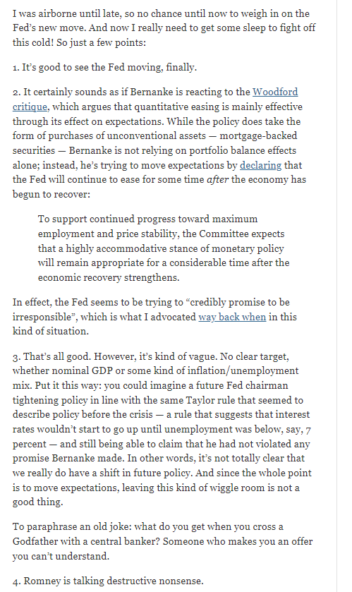
As shown in the figure, an increase in the money supply (monetary base) would result in people holding more money (excess reserve). At the moment in around 2008, the effective federal fund rate hits zero, liquidity traps started. Injecting more money (increasing the money supply) cause excess cash holding, instead of current output increase.
Forward Guidance
Forward guidance means committing to change things in the future (, with perfect credibility).
Assume that he government commits to expand money supply from /(m/) to /(m’/) in period \(t+1\) onward. Also, assume not in the liquidity trap in \(t+1\), (\(v_{t+1}=1\)). So the price level at \(t+1\) would be,
An estimated decrease in future outputs would increase \(y’u'(y’)\). However, a permanent increase in \(m’\) to keep the equation unchanged.
Forward Guidance differs from the conventional monetary policy because an extra amount of money would not be taxed back. The central bank “commits to act irresponsibly” in the future. Also, the conventional monetary policy emphasises the current money supply, but forward guidance states the future. People will know that there is no need to pay extra tax back in the future.
The is no clear downward trend of the real output while increasing money supply after getting into the liquidity trap. The market in the US implies that public sectors react to the expected decrease in future output by increasing the money supply in a long period (equivalent to the forward guidance), therefore the real output at the current period does undergo a significant decrease.
See Krugman (1988) and Eggertsson and Woodford (2003).
Here, we consider a production economy instead of an endowment economy. In this way, instead of being endowed with \(y_t\) units of the output good in each period, agents are endowed with one unit of time and they choose an inelastic supply of working.
Firms are perfectly competitive and produce output according to \(y_t=z_t l_t\), where \( z_t\) donates labour productivity and \(l_t\) the amount of labour hired.
A representative firm’s optimisation problem is then given by
$$ \max_{l_t} p_t z_t l_t- \tilde{w_t}l_t $$
F.O.C.
$$p_t z_t =\tilde{w_t} $$
The first-order condition tells that nominal wage stickiness leads to price stickiness. Given wages, \(\tilde{w_t}\), a fall in prices would reduce profits, and firms would shut down their businesses (by perfect competition assumption).
However, if prices and wages fell in equal proportion, firms would still like to hire equally many works. And the fall in prices would boost demand. P.S. the real wages keep constant.
Intuition: Firstly, as prices fall, goods get cheaper. So even 80 of spending can buy100 worth of goods. Secondly, as wages also fall, real profits are unchanged, and firms are willing to meet the additional demand. Finally, the positive impacts on \(y_t\) could offset the negative of it (from underestimated future outputs).
\( \quad \downarrow P \Rightarrow \downarrow W \Rightarrow\) unchanged profits and increase outputs
Quantitative Easing
In the open market operation, the CB purchases short-term government bonds (3-month T-bill). By QE, the CB purchases assets with longer maturity and credibility, see The Fed’s Balance Sheet, e.g. MBS.
The idea of QE is to decrease the interest rate once the short term rate is already zero, and also pool money into the market. In the recession, short term bonds’ nominal interest rates are already zero, but long term bonds may not. Thus, by purchasing long-term bonds, yields are pushed downward (real interest rate falls), and stimulate the economy. (Similar to the non-arbitrage theory). Long-term assets are equally valuable as short term assets at any horizon. In the liquidity trap, short term assets are equally valuable as holding money, so long term assets are perfect subsites to money as well (consider including liquidity premium and risk premium).
In the model with Cash in Advance and short long term assets, we consider include
A short term asset (one period) \(b_{t+1}^1\).
A long term asset (two periods), \(b_{t+1}^2\).
The price of the short-term asset is denoted \(q_t^1\), and pays out one unit of cash in period t+1.
The price of the long-term asset is denoted \(q_t^2\), and pays out one unit of cash in period t+2.
Equivalent to \( Return\ of \ LongTerm=Ro\ ShortTerm=Ro\ Cash\).
Long-term bonds are traded at arbitrage with short-term bonds which are traded at arbitrage with money.
Recall that the purpose of QE is to reduce the return on long-term bonds but that cannot be done.
If in the liquidity trap, \( x_{t+1}=0, \mu=0, i_t=0 \Rightarrow \frac{1}{q_t^1}=1 \Leftrightarrow \frac{q_{t+1}^1}{q_t^2}=1 \).
In the figure, the green curve represents QE (Fed Balance sheet). During the 2008 financial crisis and Covid-19, the Fed purchase assets (MBS and Long-term T bonds) and pay with money, in order to release liquidity into the market.
The first oil crisis started with the oil embargo proclaimed by OPEC.
OPEC: Oil exporting nations accumulated vast wealth due to the price increase. US: the oil price increase induced the recession, inflation, reduced productivity, and low economic growth.
Whyt did Keynesian economics fail in the 1970s?
According to Keynesians, the growth in the money supply can increase employment and promote economic growth. Keynesian economists believe in the Philips relationship between unemployment (economic growth) and inflation. However, both of them hiked in the 1970s.
Why did stagflation occur?
The prevailing belief has been that high levels of inflation were the result of an oil supply shock and the resulting increase in the price of gasoline, which drove the prices of everything else higher (cost-push inflation).
A now well-founded principle of economics is that excess liquidity in the money supply can lead to price inflation. Monetary policy was expansive during the 1970s, which could help explain the rampant inflation at the time.
How did Friedman work?
“Inflation is always and everywhere a monetary phenomenon.”
Milton Friedman
During the energy crisis of the 1970s, while everyone was blaming OPEC in the early part of the 70s, or the Iranian revolution in 1979, Friedman recognized who the real culprits were — Richard Nixon, who in 1973 instituted wage-price controls and, following Nixon, Gerald Ford and Jimmy Carter who continued these price controls on oil, gasoline, and natural gas.
“The present oil crisis has not been produced by the oil companies. It is a result of government mismanagement exacerbated by the Mideast war.”
– Milton Friedman, “Why Some Prices Should Rise,” Newsweek, November 19, 1973.
Friedman believed prices could not increase without an increase in the money supply. The Fed followed a constrictive monetary policy that helped drive interest rates to double-digit levels, reduce inflation.
P.S. Fed’s credibility and inflation expectation (inflation targets) also play roles in resulting in stagflation.
Inspiration
Inflation (or hyperinflation) is a monetary phenomenon by Friedman and some economists. In China’s case, stagflation seems unable to happen if there are no vast increase in money supply and loss of credibility of the central bank.
For simplification, we assume no government spending, \(g_t\), government debt, \(d_t\), and taxes, \(T_t\). Also, we assume money is stable such that \(m_t=m_{t+1}=m\) (so there is not seignorage). We here consider \(y_t\) is exogenous.
Recall
Suppose that \( y_t=u_{t+1}=…=y\), then
$$\quad 1=\beta(1+i_{t+1})\frac{p_t}{p_{t+1}}$$
Now if guess both \(x_{t+1}=x_{t+2}=0\), then the velocity of money \(v_t=1\).
\( \quad p_t=p_{t+1}=\frac{m}{y}, \quad \) and \(\quad i_{t+1}=\frac{1}{\beta}-1\geq0\)
P.S. if violate the guess \(x_{t+1}=x_{t+2}=0\), then the euler equation shows \(1+\beta (1+i_{t+1})\frac{p_t}{p_{t+1}}\) would be \( p_{t+1}=\beta p_{t}\). So, \( p_{t+1}<p_t\). By QTM \(m \cdot v_t= p_t \cdot y\) (\(m, y\) are constant), \( v_{t+1}<v_T\) must be true to make next-period price level be low than the current price level. Lower velocity means \( x_{t+2}>x_{t+1}\) (people would hoard more money on hand in the next period). The loop begins, and price level would decline in the following periods.
Here, by complementary slackness, \( x_{t+2}\times i_{t+1}=0\).
If replace \(p_{t+1}=\frac{m_{t+1} v_{t+1}}{y_{t+1}}\), =\frac{m_{t+1}}{y_{t+1}}\) by assume not in liquidity trap in the first so \(v_{t+1}=1\). Then we get,
We, in the following, assume \(x u'(x)\) is decreasing in x.
If the economy experiences a fall in period \( t+1\) output from \(y_{t+1}\) to \(y’_{t+1}\). What happens to the nominal interest rate?
We write it in this way for simplification.
u'(y)=\beta(1+i_t)\frac{p_t }{m}y’u'(y’)
As \(y_{t+1}\) decrease, \(y’u'(y’)\) increase as our assumption. The LHS keeps stable, so the interest rate has to decrease to keep the equality holding. Therefore, \(i_{t+1}\) we’ll eventually hit zero.
As \( i_{t+1}=0\), the economy enters into the liquidity trap, and people start to hoard money ,\(x_{t+1}>0\). Recall the QTM equation, \(p_t=\frac{ m_t-x_{t+1} }{y_t}=\frac{mv_t}{y} \), \(p_t\) would decrease. So, the price level at time \(t\) finally decreases as well.
From the figure, we can find that once the effective federal fund rate (The effective federal funds rate (EFFR) is calculated as a volume-weighted median of overnight federal funds transactions) hits zero, excess reserves increases. Injecting more money would only cause excess money reserves in the liquidity trap.
If future outputs decrease and price is sticky,
An extension. If the price is “sticky” in the short run. In other words, \( \bar{p}_t=\frac{m}{y}\), price cannot fall below a certain threshold. Then, a decrease in \(y_{t+1}\) would end up with decrease in current output \(y_t\). As shown in the following equation,
Future output decrease, then RHS increases, and so LHS has to increase as well. \(\frac{\partial u'(y)}{\partial y}=u”(y)\) is negative. For example, in the isoelasticity form \( u(c)=\frac{c^{1-\sigma}}{1-\sigma} \), and \(0\leq \sigma \leq1\).
In summary, recession in \(t+1\) would bring down \(y_{t+1}\). Then, firstly, decrease \(i_{t+1}\) to 0; secondly, reduce \(p_t\) to \(\bar{y}\) if price is stikcy; and thirdly, drive \(y_t\) decrease in the end. (All those are based on the guess of \(x_{t+1}=x_{t+2}=0\))
In a liquidity trap with sticky prices, outputs become “demand-driven”. The reason is that the Euler Equation is derived from the private sector, and thus \(u'(y_t)=u'(c_t)\) if not replaced with the markets clearing condition in equilibrium. The equation would then show that the increase in the LHS is driven by a decrease in consumption. A disequilibrium starts. Finally, a recession begins if nothing happened to productive capacity.
Intuition
Private sectors initially earn income, say 100, and buy goods for100 as well (Normal situation).
When they receive a “news” that income will decrease in the future from \(y_{t+1}\) to \(y’\), then they all wish to save.
However, in the aggregate, nobody can save, because noboday want to borrow or invest.
So the interest rate, as the benefits of saving, decrease to eventally zero, and private sectors start to hoard cash.
Thus, instead of spending 100, they spend80 and save $20. The demand drives down current outputs.
Role of price stickiness
Initally, current and future outputs (endownments) are all $100. \(y_{t}=y_{t+1}=100\).
A news tells us future output decrease to 80. In the current period, we save20 and spend $80. Same as the above process.
So, current spending is 80 and future spending is100.
If the price is sticky, consume $80 today and price decreases 20% at the same time. Ending up with the same amount of current consumption, \(y_t\). No recession.
If the price is sticky, then agents spend $20 fewer goods in the current. Worse off. And recession.