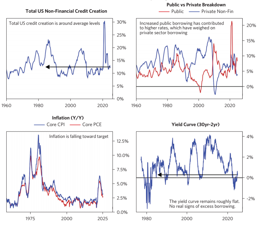
Trump Administration is widely seen as likely to increase or maintain high fiscal deficits.
To assess the impact of large deficits on yields, it is important to look at the total debt in the economy,
not just government debt.
What matters for markets and the economy is how much collective new credit is being created, and the incentive and desire of investors to buy it.
Debt Supply & Demand amount would flow to Rate. If government spending increases, then it means debt supply increases (there would be more borrowing), pushing up rate to increase.
High Borrowing -> High Rate -> Depressed the private borrowing.
Low/Normal level of credit creation would otherwise drive down inflation.
Two Cases:
Bad Scenario: Push up Inflation.
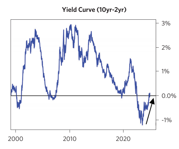
Total Debt/GDP increase (private and public debt / GDP) increase && Currency Weaken. Then Yield Curve would steepen, derived by long term rate increase, as nobody purchase the long term bond.
Think about a graph with x-axis (term), y-axis (yield), and a upward sloping curve.
Yield curve steepens.
Good Scenario (now the US situation): Do not drive up Inflation
Under this case, no buyers are buying the long-term debts.
Total Debt/GDP increases, but yield curve is flat. Public squeezes private investment. The increase in public debt does not increase private borrowing, so no extra purchasing resulted from households. Help relieve the inflation.
Yield curve flattens.
Example:
Now is the Good Scenario: The top-left figure shows the current credit creation in US is under normal level. Top-right figure shows that Public and Private debts are negative correlated. Public squeezes private, so total debt did not get up too much high.
1980s: Top-left figure shows total debts went high; Top-right figure shows public and private were positively correlated. So, bottom-left figure shows inflation hikes.
Bottom-right figure shows implicitly that the current long minus short term rate is at low level, imply that the yield curve is flat, consistent with our Good/Bad Scenario Rationale.
Supply & Supply Side of Debts
Supply Side: Currently, there are high public borrowing, and low private borrowing.
Demand Side:
Due to previous QE, Debt yield is high for investors => that would be attractive to un-levered investors, because Debts still bring enough return and less risks, attractive to people.
However, the levered investors fact different situation. As they hold debts already, high debt rate would become both their costs and returns.
The current real yield is about 2% in US, which is high relative to much of the rest of developed world. US nominal yields are at levels where the yield is attractive and diversifying relative to stocks allocation for those who need to supplement debts into their portfolio.
Again, the current yield curve is flat. For leveraged investors, they have debts liability already. Returns and Costs of debts offset.
Reference
Bridge-Water
Our Thoughts on Large US Deficits and Their Impact on Bond Yields
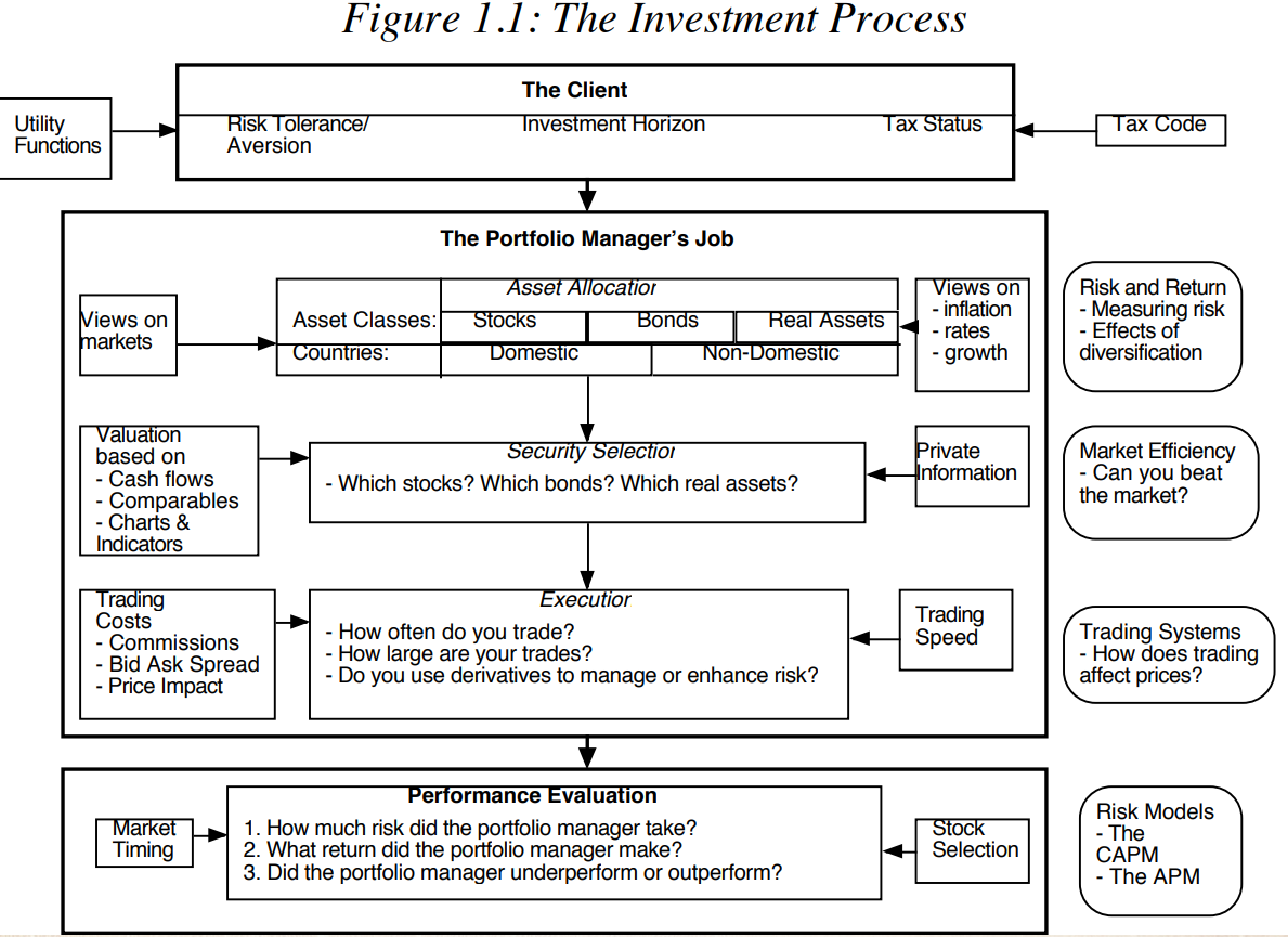
Allocating assets into different asset classes may depend on the (1) risk aversion, (2) time horizon, (3) tax status. And the (4) market timing also matters.
In other words, sensing the market timing would help you
allocate assets into different asset classes such as debts, equity;
be out of the market in the bad months, and get into the mkt in the good period.
Cost of Market Timing
Out at the wrong time. Miss the opportunity of growth, i.e..
Transaction Costs
Taxes
Market Timing Approaches
Non-financial indicators
Spurious indicators that may seem to be correlated with the market but have no rational basis.
Though there is no reasoning, there may still have some statistical pattern. Do not ignore it.
Those indicators give a sense of direction.
Feel good indicators that measure how happy investors are feeling – presumably, happier individuals will bid up higher stock prices.
The problem is that those indicators provide contemporaneous or lagging status of the market, may lack of predictability compared with the leading indicators.
Hype indicators.
Still the contemporaneous problem. Those factors tell the correlation right now, but do not have predictive power.
Also, the abnormality can be tricky when the environment is shifting.
Technical indicators, such as price charts and trading volume.
Past prices (such as price reversals or momentum, January Indicator)
Hard to say the momentum or the reversal could stay for years.
Trading Volume & Money Flow
Price increases that occur without much trading volume are viewed as less likely to carry over.
And, very heavy trading volume can also indicate the turning points in the markets.
The money flow is the difference between uptick volume and downtick volume. People find there are some predictability for longer periods, in that the equity markets overall show momentum.
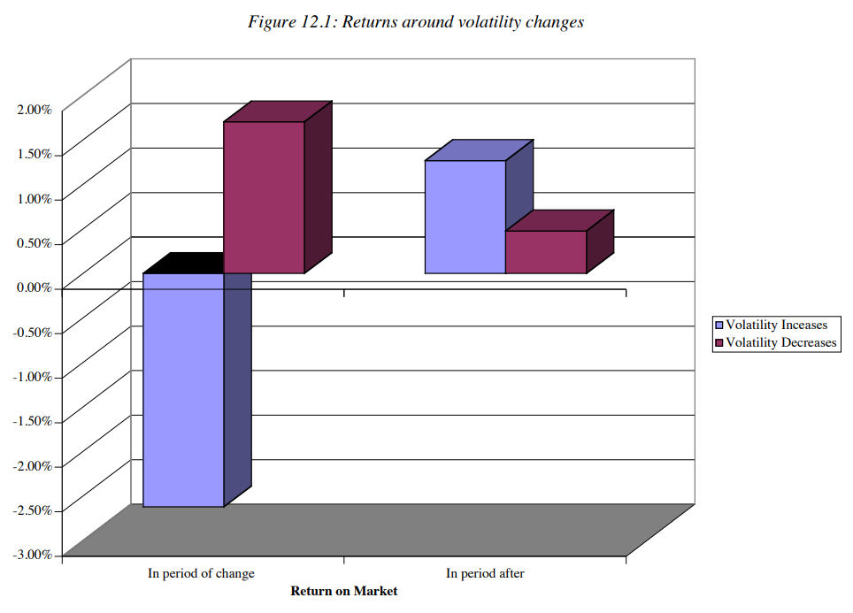
Market Volatility
Empirical research finds some evidence between the volatility change and returns.
See the blue bar: In periods that volatility increase and the market return goes down. After that period, the market is predicted to be like volatility increase and market return goes up.
Purple bar: in periods of volatility decrease and market return increase, the following period may have less volatility decrease and still returns.
Other price and sentiment indicators
Chart Patterns: supports and resistance lines are used to determine when to move in and out of individual stocks.
Sentiment indicators: measure the mood of the market.
Trader sentiments
Mean Reversion indicators, where stocks and bonds are viewed as mis-priced if they trade outside what is viewed as a normal range.
That approach is based on the assumption that stock price would revert to the P/E, and debt return would revert back certain interest rate.
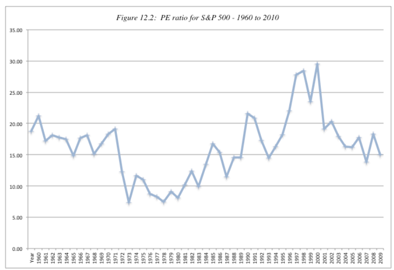
P/E (see figure below for the normal range of P/E ratio)
If stock is above or below the normal P/E, then it is overvalued or undervalued. The median is around 16.
The P/E might go abnormally high in recession, not only because (1) the stocks are overvalued, but also because (2) the earnings are dropped down during recession.
Rate performs similarly.
\Delta Interest Rate_t = 0.0139 – 0.1456 InterestRate_{t-1}, where R^2=0.728. Coefficients are significant.
The regression suggest two things:
Change in interest rates in the period is negatively correlated with the level of rates at the end of each prior year.
The speed shrinks. For every 1% increase in the level of current rate, the expected drop in interest rate in the next periods increases by 0.1456%.
Fundamentals
Using the fundamentals to predict market timing is to focus on macroeconomic variables such as interest rate, inflation and GNP growth and devise investing rules based upon the levels or changes in macro economic variables.
Two keys of using this approach. (to build up the logic chain of prediction)
Get handle how the market reacts as macro econ fundamentals change.
Get good predictions of changes in macro econ fundamentals.
Macro economic variables, such as the level of interest rate or the state of the econ cycle.
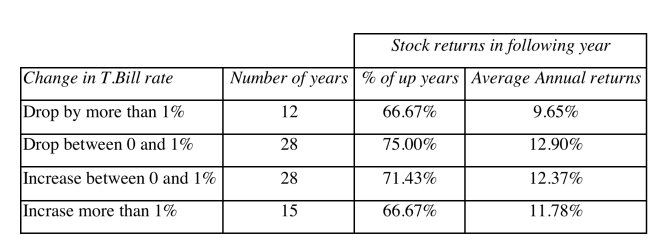
There are some common sense that the following changes would indicate the increase in stock price:
Buy when Treasury bill rates are low, will end up with growth of stock price.
Buy when Treasury bond rates have dropped, will end up with growth of stock price.
Buy GNP growth is strong, will end up with growth of stock price.
However, empirical evidence shows the other way. For example, the table below shows T-bill rate drops or increases could both contribute to the increase in Annual returns.
Valuing the Market
Just as you can value individual stocks with intrinsic valuation (DCF) models and relative valuation (multiples) models, you can value the market as well. If the valuation is faithful, you can reply on it to predict the market timing.
Intrinsic valuation that apply to the mkt. <- depends on assumptions and inputs.
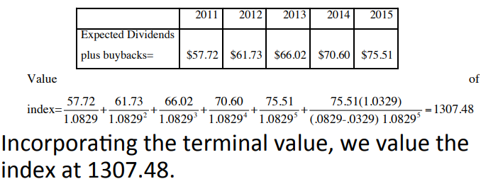
Use the S&P500 price and the index’s dividends to do the DCF.
INPUTs: (1) S&P500 price, 1257.64 at 2011(2) Dividends and buyback on the index amount over previous year, 53.96 (3) expected earning growth for the following 5 years, 6.95% (4) expected growth of the economy (set as risk free rate) 3.29%, (5) treasury bond rate, plus the market risk premium (set it yourself) 5% to get the cost of equity 3.29%+5%=8.29%. Then, do the DCF
Relative Valuation <- value a market relative to other market, or across years.
Other methods, such as run regression on P/E to T-bill to find correlation.
Does the Market Timing Work?
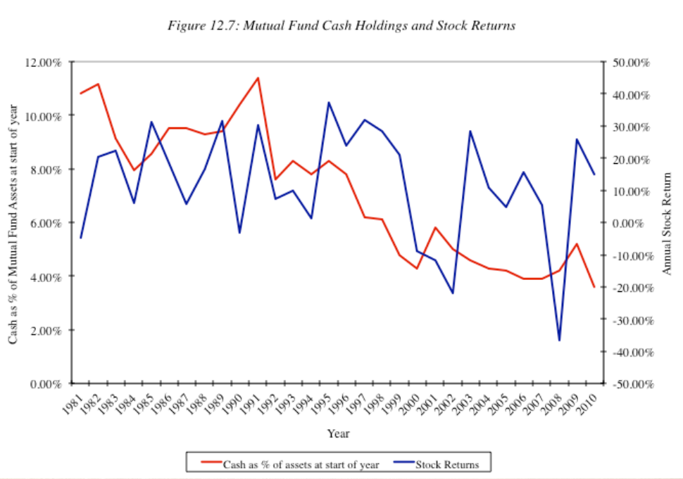
Mutual Fund Managers: constantly try to time the markets by changing the amount of cash that they hold in the fund. If expected bullish, then cash balances decreases, vice versa.
They call timing the market as Tactical Asset Allocation, TAA.
See figure below, empirical evidence shows they do predict the market by changing the cash position.
Investment Newsletter: often take bullish or bearish view about the market.
There is continuity on Newsletter way. Investment newsletters that give bad advice on market timing are more likely to continue to give bad advice than are newsletters that gave good advice to continue giving good advice. In other words, it depend on the writer’s ability.
Market strategists: make forecast for the overall market.
Professor Market Timers provide advice, however, their decision works for very short time, and only work for private clients.
Market Timing Strategies
Adjust Asset Allocation: change across asset classes
Switch Investment Styles: change within asset classes but different styles, such as from growth to value.
Sector Rotation: with in asset classes, but different sector.
Market Speculation.
Market Timing Instruments
Futures Contracts
Options Contracts
ETFs
Implications and Insights
Overall, it’s good summary and a Beginner’s Tutorial, but not include technical implementation method, instruction, or philosophy.
Cycles Factors, as the below three, generate the cycle. (, are marked by wars. Starting the cycle at the end of WW II.)
Internal Order – Productivity increase
Debt raises relative to Incomes. (Debt is money, and debt means more buying power.) Increase the gaps of wealth, -> Internal Conflicts start to emerge
External Conflict:
Climates, and Technologies (Mans inventiveness, new technologies)
Apply those five factors into the current world.
The current Debt Climate condition:
Currently,
Private debt sectors (individuals) get more and more indebted.
Public debt sector take on the debt, and the central bank is supporting that effort.
On a cyclical basis, total debt relative to GDP continuing to rise near its high.
Debt service cost (a function of interest rate) increase, and public sector takes the burden.
Then, Public sector starts to get indebtedness.
That is the short-term cycle.
The cycle for development, Ray considers there are four stages.
A poor country that has no capital accumulation starts to recognise the poverty.
Country gets money to get capital formation, and conduct infrastructure (such as build roads). Do not waste that money, and put money into productive uses.
Mentality. As the country getting richer, it still think it is not rich enough, is still poor.
The country keeps getting richer, and start to realise it do not have to work that hard, and start to enjoy the life.
As there are less works, the country gets poor, but still think itself is rich. So start to borrow money.
How to create a portfolio.
has a diversified portfolio that is able to absorb risks and unforeseen.
The types of assets in the portfolio might include
Inflation index bonds
Gold
Real Rates
Avoid the credit risk. (The above three are the government obligations, so less credit risks are there)
Such as, we short Inflation index bond and long Gold (we could avoid the credit risks, and diversify the portfolio with certain target)
The Paris Club (Club de Paris, 巴黎俱乐部) has reached 478 agreements with 102 different debtor countries. Since 1956, the debt treated in the framework of Paris Club agreements amounts to $ 614 billion.
Low-income countries generally do not have access to these markets. The assistance from bilateral and multilateral donors remains vital for them. Non-Paris Club creditors are becoming an increasingly important source of financing for these countries. Yet despite the fact that Paris Club creditors now have to deal with far more complex and diverse debt situations than in 1956, their original principles still stand.
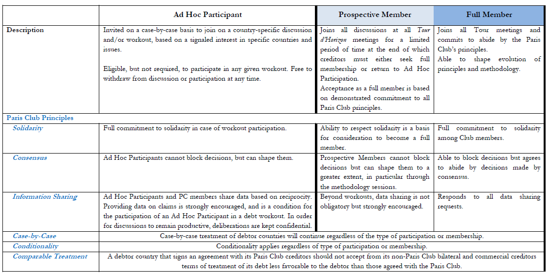
Members
Duty of Members
Permanent Members
The 22 Paris Club permanent members are countries with large exposure to other States woldwide and that agree on the main principles and rules of the Paris Club. The claims may be held directly by the government or through its appropriate institutions, especially Export credit agencies. These creditor countries have constantly applied the terms defined in the Paris Club Agreed Minutes to their bilateral claims and have settled any bilateral disputes or arrears with Paris Club countries, if any. The following countries are permanent Paris Club members:
Other official creditors can also actively participate in negotiation sessions or in monthly “Tours d’Horizon” discussions, subject to the agreement of permanent members and of the debtor country. When participating in Paris Club discussions, invited creditors act in good faith and abide by the practices described in the table below. The following creditors have participated as creditors in some Paris Club agreements or Tours d’Horizon in an ad hoc manner:
In 1956, the world economy was emerging from the aftermath of the Second World War. The Bretton Woods institutions were in the early stages of their existence, international capital flows were scarce, and exchange rates were fixed. Few African countries were independent and the world was divided along Cold War lines. Yet there was a strong spirit of international cooperation in the Western world and, when Argentina voiced the need to meet its sovereign creditors to prevent a default, France offered to host an exceptional three-day meeting in Paris that took place from 14 to 16 May 1956.
Dealing with the Debt Crisis (1981-1996)
1981 marked a turning point in Paris Club activity. The number of agreements concluded per year rose to more than ten and even to 24 in 1989. This was the famous “debt crisis” of the 1980s, triggered by Mexico defaulting on its sovereign debt in 1982 and followed by a long period during which many countries negotiated multiple debt agreements with the Paris Club, mainly in sub-Saharan Africa and Latin America, but also in Asia (the Philippines), the Middle East (Egypt and Jordan) and Eastern Europe (Poland, Yugoslavia and Bulgaria). Following the collapse of the Soviet Union in 1992, Russia joined the list of countries that have concluded an agreement with the Paris Club. So by the 1990s, Paris Club activity had become truly international.
Debt Burden Enlarges for some Countries
In 1996, the international financial community realized that the external debt situation of a number of mostly African low-income countries had become extremely difficult. This was the starting point of the Heavily Indebted Poor Countries (HIPC) Initiative.
The HIPC Initiative demonstrated the need for creditors to take a more tailored approach when deciding on debt treatment for debtor countries. Hence in October 2003, Paris Club creditors adopted a new approach to non-HIPCs: the “Evian Approach”.
Evian Approach
General frame of the Evian approach
Analysis the sustability
When a country approaches the Paris Club, the sustainability of its debt would be examined, before the financing assurances are requested, in coordination with the IMF according to its standard debt sustainability analysis to see whether there might be a sustainability concern in addition to financing needs. Specific attention would be paid to the evolution of debt ratios over time as well as to the debtor country’s economic potential; its efforts to adjust fiscal policy; the existence, durability and magnitude of an external shock; the assumptions and variables underlying the IMF baseline scenario; the debtor’s previous recourse to Paris Club and the likelihood of future recourse. If a sustainability issue is identified, Paris Club creditors will develop their own view on the debt sustainability analysis in close coordination with the IMF.
if face liquidity problem
For countries who face a liquidity problem but are considered to have sustainable debt going forward, the Paris Club would design debt treatments on the basis of the existing terms. However, Paris Club creditors agreed that the rationale for the eligibility to these terms would be carefully examined, and that all the range built-into the terms including through shorter grace period and maturities, would be used to adapt the debt treatment to the financial situation of the debtor country. Countries with the most serious debt problems will be dealt with more effectively under the new options for debt treatments. For other countries, the most generous implementation of existing terms would only be used when justified.
if not sustainable or need special treatment
For countries whose debt has been agreed by the IMF and the Paris Club creditor countries to be unsustainable, who are committed to policies that will secure an exit from the Paris Club in the framework of their IMF arrangements, and who will seek comparable treatment from their other external creditors, including the private sector, Paris Club creditors agreed that they would participate in a comprehensive debt treatment. However, according to usual Paris Club practices, eligibility to a comprehensive debt treatment is to be decided on a case-by-case basis.
In such cases, debt treatment would be delivered according to a specific process designed to maintain a strong link with economic performance and public debt management. The process could have three stages. In the first stage, the country would have a first IMF arrangement and the Paris Club would grant a flow treatment. This stage, whose length could range from one to three years according to the past performance of the debtor country, would enable the debtor country to establish a satisfactory track record in implementing an IMF program and in paying Paris Club creditors. In the second stage, the country would have a second arrangement with the IMF and could receive the first phase of an exit treatment granted by the Paris Club. In the third stage, the Paris Club could complete the exit treatment based on the full implementation of the successor IMF program and a satisfactory payment record with the Paris Club. The country would thus only fully benefit from the exit treatment if it maintains its track record over time.
Data
There data in the website yoy.
Insights
Refer to Horn et al., (2021) figure 9 in page 13, Paris Club seems played important role during 2010s.
I have passed the CFA III level exam, and been granted the chart.
For any errates and insights, please free to contact to me.
Here below are my learning footprints for CFA level III. All files are converted to .html as you will find in the following . If you need the raw markdown codes, please move to my Github Repo.
P.S. there are typos and miswritten parts in the notes. Welcome to find me and help me update those mistakes. Or, probably I will update them if I fail the level III exam (in that I would review those notes). 🙂
The first approach is that analysts focus on flows of export and imports to establish what the net trade flows are and how large they are relative to the economy and other, potentially larger financing and investment flows. The approach also considers differences between domestic and foreign inflation rates that relate to the concept of purchasing power parity. Under PPP, the expected percentage change in the exchange rate should equal the difference between inflation rates. The approach also considers the sustainability of current account imbalances, reflecting the difference between national saving and investment.
The second approach is that the analysis focuses on capital flows and the degree of capital mobility. It assumes that capital seeks the highest risk-adjusted return. The expected changes in the exchange rate will reflect the differences in the respective countries’ assets’ characteristics such as relative short-term interest rates, term, credit, equity and liquidity premiums. The approach also considers hot money flows and the fact that exchange rates provide an across the board mechanism for adjusting the relative sizes of each country’s portfolio of assets.
, where C_{i,j} are scalars and v_i\in \mathbb{R} is the measurement noise. The noise is unknown, while we assume it follows certain patterns (the assumptions are due to some statistical properties of the noise). We assume v_i, v_j are independent for i\neq j. Properties are mean of zero, and variance equals sigma squared.
$$\mathbb{E}(v_i)=0$$
$$\mathbb{E}(v_i^2) = \sigma_i^2$$
We can rewrite y_i = \sum_{j=1}^n C_{i,j} x_j +v_i as,
We solve for the least squared estimator from the optimisation problem, (there is a squared L2 norm)
$$ \min_x || y-Cx ||_2^2 $$
Recursive Least Squared Method
The classic least squared estimator might not work well when data evolving. So, there emerges a Recursive Least Squared Method to deal with the discrete-time instance. Let’s say, for a discrete-time instance k, y_k \in \mathbb{R}’ is within a set of measurements group follows,
$$y_k = C_k x + v_k$$
, where C_k \in \mathbb{R}^{l\times n}, and v_k \in \mathbb{R}^l is the measurement noise vector. We assume that the covariance of the measurement noise is given by,
$$ \mathbb{E}[v_k v_k^T] = R_k$$
, and
$$\mathbb{E}[v_k]=0$$
The recursive least squared method has the following form in this section,
, where \hat{x}k and \hat{x}{k-1} are the estimates of the vector x at the discrete-time instants k and k-1, and K_k \in \mathbb{R}^{n\times l} is the gain matrix that we need to determine. K_k is coined the ‘Gain Matrix’
The above equation updates the estimate of x at the time instant k on the basis of the estimate \hat{x}_{k-1} at the previous time instant k-1 and on the basis of the measurement y_k obtained at the time instant k, as well as on the basis of the gain matrix K_k computed at the time instant k.
$P_k = \mathbb{E}(\epsilon_k \epsilon_k^T)$, and $P_{k-1} = \mathbb{E}(\epsilon_{k-1} \epsilon_{k-1}^T)$.
$\mathbb{E}(\epsilon_{k-1} v_k^T) = \mathbb{E}(\epsilon_{k-1}) \mathbb{E}(v_k^T) =0$ by the white noise property of $\epsilon$ and $v$. However, $\mathbb{E}(v_k v_k^T) = R_k$. Substituting all those into $P_k$, we would get,
We take F.O.C. to solve for K_k = arg\min_{K_k} W_k = tr\bigg( \mathbb{E}(\epsilon_k \epsilon_k^T ) \bigg) = tr(P_k), by letting \frac{\partial W_k}{\partial K_k} = 0. See the Matrix Cookbook and find how to do derivatives w.r.t. K_k.
Sigmoid function is largely used for the binary classification, in either machine learning algorithm or econometrics.
Why the Sigmoid Function shapes in this form?
Firstly, let’s introduce the odds.
Odds provide a measure of the likelihood of a particular outcome. They are calculated as the ratio of the number of outcomes that produce that outcome to the number that do not.
Odds also have a simple relation with probability: the odds of an outcome are the ratio of the probability that the outcome occurs to the probability that the outcome does not occur. In mathematical terms, p is the probability of the outcome, and 1-p is the probability of not occurring.
$$ odds = \frac{p}{1-p} $$
Odd and Probability
Let’s find some insights behind the probability and the odd. Probability links with the outcomes in that for each outcomes, the probability give its specific corresponding probability. Pr(Y), where Y is the outcome, and Pr(\cdot) is the probability density function that project outcomes to it’s prob.
What about the odds? Odds is more like a ratio that is calculated by the probability as the formula says.
Implication: Compared to the probability, odds provide more about how the binary classification is balanced or not, but the probability distribution.
Example
Rolling a six-side die. The probability of rolling 6 is 1/6, but the odd is $1/5.
Formula
$$ odd = \frac{Pr(Y)}{1-Pr(Y)} $$
, where Y is the outcomes.
Logit
As the probability Pr(Y) is always between [0,1], the odds must be non-negative, odd \in [0,\infty]. We may want to apply a monotonic transformation to re-gauge that range of odds. We will apply on the logarithm.
As the transformation we apply on is monotonic, the Sigmoid function remains the similar properties as the odd. The Sigmoid function keeps the similar implication, representing the balance of the binary outcomes.
Then, we bridge Y = f(X), the outcome Y is a function of events X. Here, we assume a linear form as Y = X\beta. The sigmoid function would then become a function of X.
At x=x’ the Dirac Delta function is sometimes thought of has having an “infinite” value. So, the Dirac Delta function is a function that is zero everywhere except one point and at that point it can be thought of as either undefined or as having an “infinite” value.
$\tilde{P}(\omega)$ is the risk-neutral probability measure.
${P}(\omega)$ is the actual probability measure.
Properties:
$Z(\omega)>0$
$\mathbb{E}(Z)=1$
As \tilde{P}(\omega) = Z(\omega) P(\omega), so if Z(\omega), then \tilde{P}(\omega)>P(\omega). vice versa.
We can calculate that,
$$ \underbrace{\tilde{\mathbb{E}}(X)}_{\text{Expectation under Risk-neutral Probability Measure}} = \underbrace{\mathbb{E}(ZX)}_{\text{Expectation under Actual Probability Measure}} $$
Proof & Example
Under (\Omega,\mathcal{F},P), A\in \mathcal{F}, let X be a random variable X\sim N(0,1). \mathbb{E}(X)=0, and \mathbb{Var}(X)=1.
$Y=X+\theta$, $\mathbb{E}(Y)=\theta$, and $\mathbb{Var}(Y)=1$.
$X$ here is s.d. normal under the actual probability measure.
However, Y here is not standard normal under the current probability P(.), because \mathbb{E}(Y)\neq0.
What do we do?
We change the probability measure from P(.)\to\tilde{P}(.) to let Y be standard normal under the new probability measure!