Category: Economic Growth

Ramsey (1928), followed much later by Cass (1965) and Koopmans (1965), formulated the canonical model of optimal growth for an economy with exogenous ‘labour augmenting technological progress. The R.C.K model (or called. Ramsey (Neo-classical model) can be considered as an extension of the Solow model but without an assumption of a constant exogenous saving rate.

Assumptions

Firms

1. Identical Firms.
2. Markets, factors markets and outputs markets, are competitive.
3. Profits distributed to households.
4. Production fucntion with labour augmented techonological progress, \(Y=F(K,AL)\). (Three properties of the production: 1. CRTS; 2. Diminishing Outputs, second derivative<0; 3. Inada Condition.)
5. \(A\) is same as in Solow model, \(\frac{\dot{A}}{A}=g\). Techonology grows at an exogenous rate “g”.

Households

1. Identical households.
2. Number of households grows at “n”.
3. Households supply labour, supply capital (borrowed by firms).
4. The initial capital holdings is \(\frac{K(0)}{H}\)., where \(K(0)\) is the initial capital, and \(H\) is the initial number of households.
5. Assume no depreciation of capital.
6. Households maximise their lifetime utility.
7. The utility fucntion is constant-relative-risk-aversion (CRRA).

The lifetime utility for a certain household is represented by,

$$ U=\int_{t=0}^{\infty} e^{-\rho t}\cdot u(C(t))\cdot\frac{L(t)}{H} dt$$

Behaviours

Firms

By CRTS, \(\frac{\partial F(K,AL)}{\partial K}=\frac{\partial f(k)}{\partial k}\).

$$ F(K,AL)=AL\cdot F(\frac{K}{AL},1) \quad \text{By CRTS} $$

$$ \frac{\partial F(K,AL)}{\partial K}= AL \cdot \frac{\partial F(K/AL,1)}{\partial K}\cdot \frac{\partial K/AL}{\partial K}=F'(K/AL,1)\\=f'(k) $$

For the firms’ problem, the market is competitive, firms maximise their profits, then we get capital earns its marginal products,

$$ r(t)=\frac{\partial F(K,AL))}{\partial K}=f'(k(t)) $$

Similarly, labours earns its marginal products,

$$ W(t)=\frac{\partial F(K,AL)}{\partial L}=\frac{\partial F(K,AL)}{\partial AL}\cdot \frac{\partial AL}{L} $$

$$ =A \frac{\partial F(K,AL)}{\partial AL} =A \frac{\partial ALF(K/AL,1)}{\partial AL} $$

Apply the chain rule and replace \(F(K/AL,1)=f(k)\) and \(F'(K/AL,1)=f'(k)\). Then, we would get,

$$ W(t)=A[f(k)-kf'(k)]\ or\ W(t)=A(t)[f(k(t))-k(t)f'(k(t))]$$

We denote \(w(t)=W(t)/A(t)\) as the efficient wage rate, then we get,

$$ w(t)=f(k(t))-k(t)f'(k(t)) $$

Another key assumption of this model is,

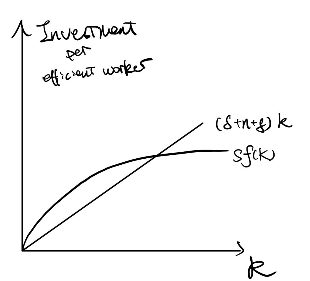
$$ \dot{k}(t)=f(k(t))-c(t)-(n+g)k(t) $$

, which represents the actual investment (outputs minus consumptions), \(f(k(t))-c(t)\); and break-even investment, \((n+g)k(t)\). The implication is that population growth and technology progress would dilute the capital per efficient work.

The difference with the Solow model is that we do not assume constant saving rate “s” in \(sf(k)\) now, instead we assume the investment as \(f(k)-c\).

Households

The budget constraint of households is that: the PV of lifetime consumption cannot exceed the initial wealth and the lifetime labour incomes.

\int_{t=0}^{\infty} e^{-R(t)}\cdot C(t) \cdot \frac{L(t)}{H} dt \leq \frac{K(0)}{H}+\int_{t=0}^{\infty} e^{-R(t)}\cdot W(t) \cdot \frac{L(t)}{H} dt

, where \(R(t):=\int_{\tau=0}^ t r(\tau) d\tau\) to represent the discount rate overtime. When \(r\) is a constant, \(R(t)=r\cdot t\) and \(A(t)=A(0)e^{rt}=A(0)e^{R(t)}\).

The budget constraint can be rewritten as,

$$ \frac{K(0)}{H}+\int_{t=0}^{\infty} e^{-R(t)}\cdot[W(t)-C(t)]\cdot \frac{L(t)}{H} dt \geq 0 $$

And easy to know,

$$ \lim_{s\rightarrow \infty} [ \frac{K(0)}{H}+\int_{t=0}^{s} e^{-R(t)}\cdot[W(t)-C(t)]\cdot \frac{L(t)}{H} dt ] $$

$$ e^{-R(s)}\frac{K(s)}{H}= \frac{K(0)}{H}+\int_{t=0}^{\infty} e^{-R(t)}\cdot[W(t)-C(t)]\cdot \frac{L(t)}{H} dt $$

We get the non-Ponzi condition,

$$ \lim_{s\rightarrow \infty} \frac{K(s)}{H}\geq 0 $$

Then,

$$ \frac{K(s)}{H}=e^{R(s)}[ \frac{K(0)}{H}+\int_{t=0}^{\infty} e^{-R(t)}\cdot[W(t)-C(t)]\cdot \frac{L(t)}{H} dt] $$

Maximisation of Households’ Problem

We plug the \( \begin{cases} C(t)=A(t)c(t)\\L(t)=L(0)e^{nt}\\A(t)=A(0)e^{gt} \end{cases} \) into households’ lifetime utility function (objective function), and then get the,

$$ U=B\cdot \int_{t=0}^{\infty} e^{-\beta t} \frac{c(t)^{1-\theta}}{1-\theta} dt $$

, where \(B:=A(0)^{1-\theta} \frac{L(0)}{H}\) and \(\beta:=\rho-n-(1-\theta)g\) (we need \(\beta>0\) to make the utility function convergence), and the utility function is, \(u(c_t)=\frac{c_t^{1-\theta}}{1-\theta}\).

The budget constraint is the households’ lifetime budget constraints divided by \(A(0)\) and \(L(0)\),

$$ k(0)+\int_{t=0}^{\infty} e^{-R(t)}\cdot[w(t)-c(t)]\cdot e^{(g+n)t} dt \geq 0 $$

Lagrangian

$$ \mathcal{L}=B\cdot \int_{t=0}^{\infty} e^{-\beta t}\frac{c_t^{1-\theta}}{1-\theta} dt\\ +\lambda [k_0+\int_{t=0}^{\infty} e^{-R(t)}(w_t-c_t) e^{(n+g)t}dt ]$$

F.O.C.

$$B \cdot e^{-\beta t} c_t^{-\theta}=\lambda \cdot e^{-R(t)+(n+g)t} $$

Take logritham,

$$ ln(B)-\beta t-\theta ln(c_t)=ln(\lambda)-R(t)+(n+g)t $$

$$ ln(B)-\beta t-\theta ln(c_t)=ln(\lambda)-\int_{\tau=0}^t r(\tau) d\tau+(n+g)t $$

Thus, we get the relationship between consumption, \(c_t\), and \(R(t)\). Later, we take differentiation w.r.t. \(t\), and we would get,

$$ -\beta -\theta \frac{\dot{c_t}}{c_t} =-r(t)+n+g$$

So, (by replacing in the \(\beta\))

$$ \frac{\dot{c_t}}{c_t}=\frac{r(t)-n-g-\beta}{\theta}=\frac{r(t)-\rho-\theta g}{\theta}$$

Therefore, we get the time-path of consumption.

Dynamics

The dynamics of consumption

Combine the firms’ problems and households’ problems.

$$ \begin{cases} \frac{\dot{c_t}}{c_t}=\frac{r(t)-\rho-\theta g}{\theta} \\ r(t)=f'(k(t)) \end{cases} \Rightarrow \frac{\dot{c_t}}{c_t}=\frac{ f'(k(t)) -\rho-\theta g}{\theta} $$

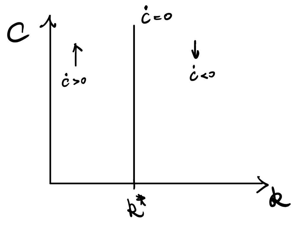
Therefore, we find the time-path of consumption depends on \(f'(k)\). We define \(k*\) is the solution when \(f'(k)=\rho+\theta g\). So, at \(k^*\), the numerator of RHS equals zero.

As \(f(k)\) is an increasing function but with diminishing returns, so \(f”(k)<0\) and that means \(f'(k)\) is a decreasing function in k. Thus,

• at \(k<k^*\), \(f(k)>\rho+\theta g\) and \( \frac{\dot{c_t}}{c_t} >0\);
• at \(k>k^*\), \(f(k)<\rho+\theta g\) and \( \frac{\dot{c_t}}{c_t} <0\).

The dynamics of k

We recall the assumption,

$$ \dot{k}(t)=f(k(t))-c(t)-(n+g)k(t) $$

At \(\dot{k}=0\), consumption, \(c(t)=f(k(t))-(n+g)k(t)\), equals outputs minus break-even investment.

We now consider the Solow model without the depreciation term. Recall the difference between the RCK model and the Solow model is that we do not assume a constant saving rate over time, but other things keep similar. Thus, the term \(c(t)\) is “equivalent” to \(sy\) in Solow model.

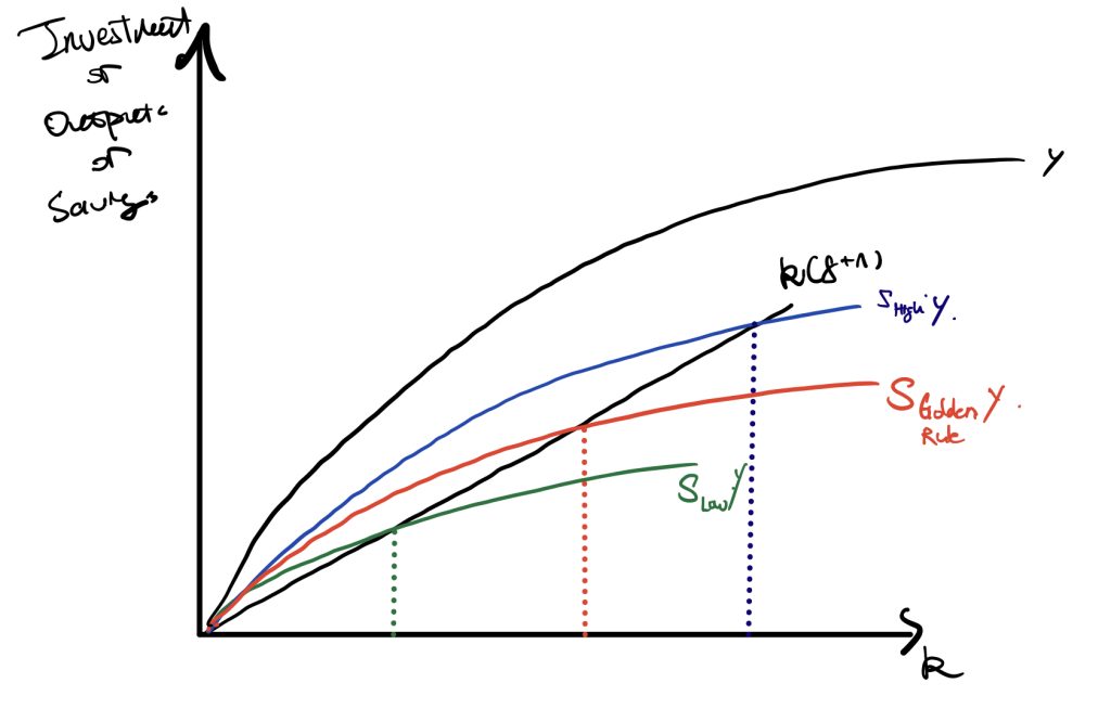
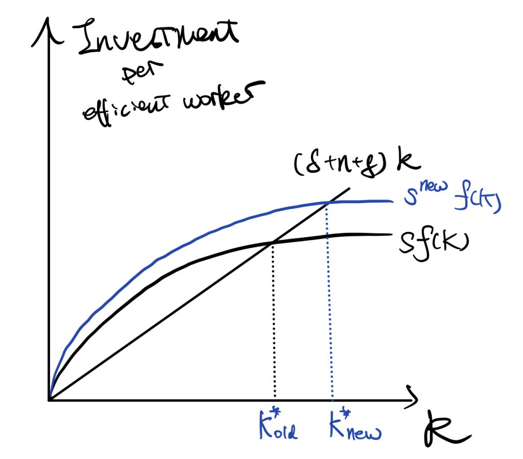
In the Solow model, changes in saving rate would change the magnitude of \(sy\) curve. The Golden Rule saving rate is “s” that maximises consumption (the difference between Y and the interaction between \(sy\) and \(k(g+n)\)). The shape of the production function determines the property of the Golden Rule saving rate.

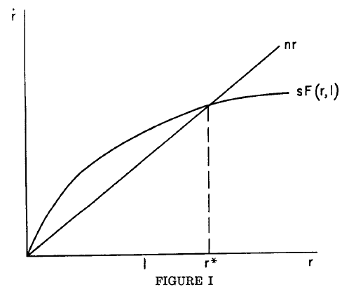
An equilibrium level of consumption is determined in mainly two steps. 1. the interaction between saving \(sy\) and \((n+g)k\) determines the \(k^*\). 2. plug \(k^*\) back to \(sy\) and find the difference between outputs and savings to get consumption.

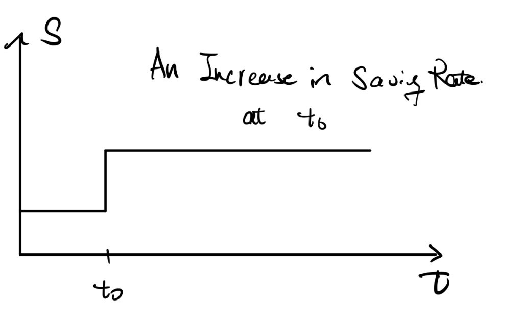
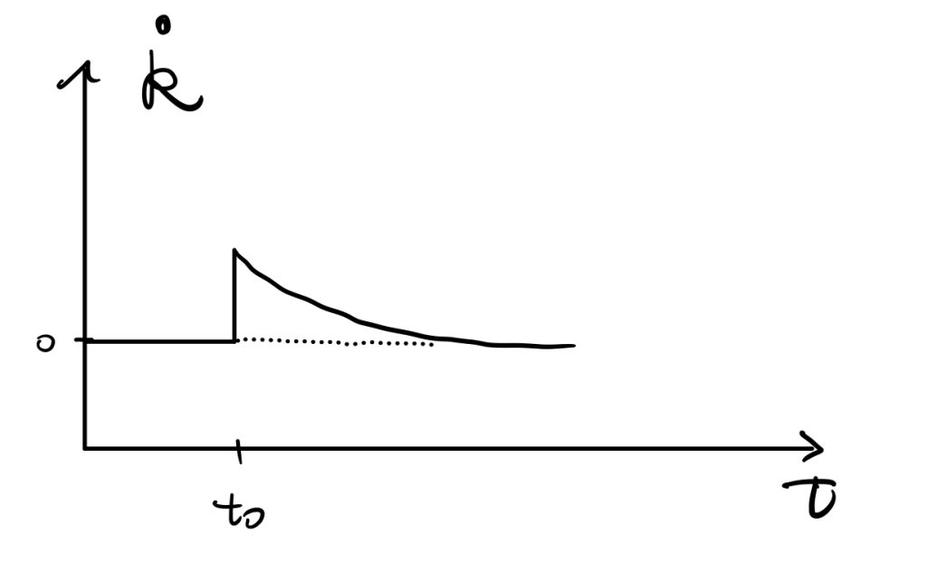
We here focus on the second step, the equilibrium level of \(k^*\) determines consumption and thus consumption is a function of \(k^*\). At a lower saving rate (see Figure 2), \(k^*\) is too small, so there is less consumption. At a higher saving rate, \(k^*\) is too large, so there is also less consumption. Therefore, we can find that consumption is in a quadratic form w.r.t. \(k^*\).

$$ (s\downarrow) \Leftrightarrow k \downarrow \to c \downarrow$$

$$ (s\uparrow) \Leftrightarrow k \uparrow \to c \downarrow$$

$$ (s_{GoldenRule}) \Leftrightarrow k^*\to c_{max}$$

Or, we can consider consumption as the difference between \(y\) and \((n+g)k\). The wedge like area gets large and then shrinks.

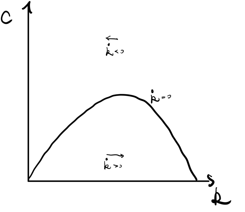
Overall, the above facts make the \(\dot{k}=0\) curve.

Recall \( \dot{k}(t)=f(k(t))-c(t)-(n+g)k(t) \).

Above the curve where \(c\) is large, then \(\dot{k}<0\) so \(k\) decreases. Below the curve where \(c\) is small, then \(\dot{k}>0\) so \(k\) increases. Implication is that if less consumption, then more saving, \(\dot{k}\) increases.

Phase Diagram.

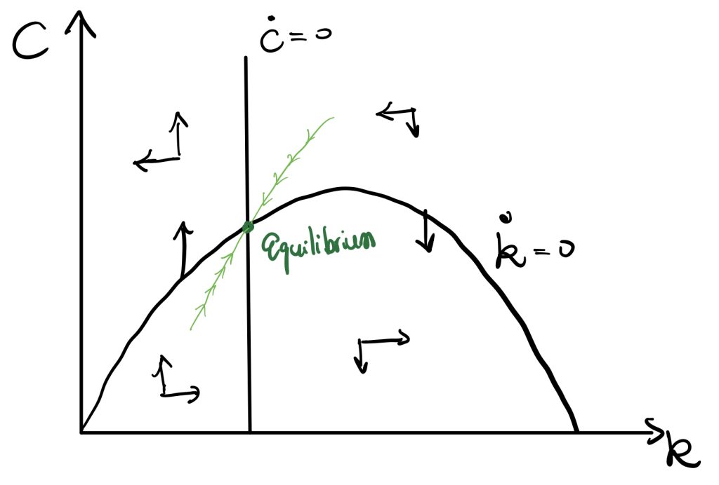
Combining Figure 1 and Figure 3, we get the above Phase Diagram. The equilibrium is shown in the figure above.

P.S. We can prove that the equilibrium is less than Golden Rule level \(k^*_{GoldenRule}\) (which is the maximum point in the quadratic shaped curve). The proof is the following,

The value of k at \(\dot{c}=0\) is \(f'(k)-\rho-\theta g=0\), and the Golden Rule level is \(c=f(k)-(n+g)k\) (as we illustrated before), and take f.o.c. w.r.t. k to solve the Golden rule k. \(\frac{\partial c}{\partial k}=0 \to f'(k)=n+g\). Therefore, we get,

$$ \begin{cases} f_1:=f'(k_{equilibrium})=\rho+\theta g \quad\text{equilibrium in phase diagram}\\ f_2:=f'(k_{GoldenRule})=n+g\quad\text{golden rule level}\end{cases}$$

$$ \rho+\theta g>n+g \quad \text{by our assumption of \beta convergence}$$

So, we get,

$$ f_1>f_2 $$

$$ k_{equilibrium}< k_{GoldenRule} $$

Thus, we find the equilibrium level capital per efficient workers, \(k_{equilibrium}\), must be less than the Golden Rule level \( k_{GoldenRule} \).

From the phase diagram, we can get the saddle path that can achieve equilibrium.

BGP

At the Balanced Growth Path, the economy is in equilibrium. So the time-paths satisfy \( \frac{\dot{c}}{c}=0, and \frac{\dot{k}}{k}=0 \). Therefore, we can get the BGP of others,

$$y=k^{\alpha}\to lny=\alpha ln(k)\to \frac{\dot{y}}{y}= \alpha\frac{\dot{k}}{k}=0 $$

$$y=\frac{Y}{AL}\to lny=lnY-lnA-lnL\to \frac{\dot{y}}{y}=0= \frac{\dot{Y}}{Y}- (g+n)\\ \Rightarrow \frac{\dot{Y}}{Y}= g+n $$

$$ \frac{\dot{c}}{c}=0\to c=\frac{C}{AL} \to \frac{\dot{c}}{c} =g+n $$

Similarly (also as the similar method in Solow model), we can get,

$$ \begin{cases} \frac{\dot{Y}}{Y}=n+g \\ \frac{\dot{C}}{C}=n+g \\ \frac{\dot{K/L}}{K/L}=g \\ \frac{\dot{Y/L}}{Y/L}=g \\ \frac{\dot{C/L}}{C/L}=g \end{cases} $$

Fiscal Policy

Assumption: government conducts government purchases, \(G(t)\). The government purchases do not affect the utility of private sectors, and future outputs. Government finances, G(t), by lump-sum taxes.

We can consider the crowding-out effect. Under full employment, government purchases take away part of the consumptions. In our case, government spending takes away some of the savings. Therefore, the dynamics of capital per efficient workers become (the minus government spending term shifts the curve downward by G(t)),

$$\dot{k}(t)=f(k(t))-c(t)-G(t)-(n+g)k(t)$$

In short, government purchases would make the economy achieve a new equilibrium where there is less consumption but the same capital (investment from the private sector) level. Also, the saddle path moves downward.

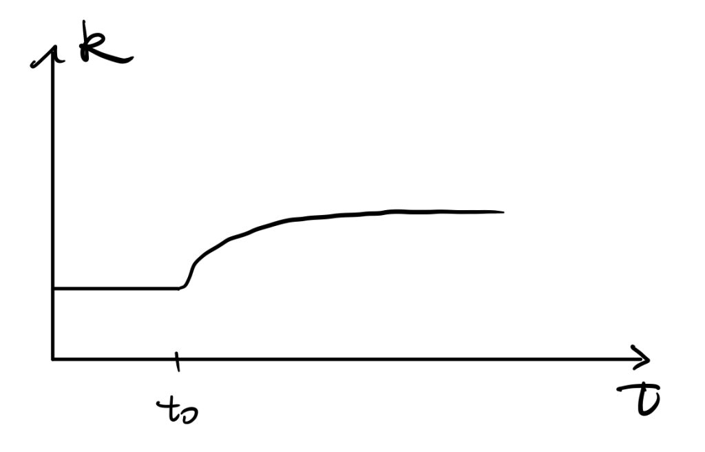
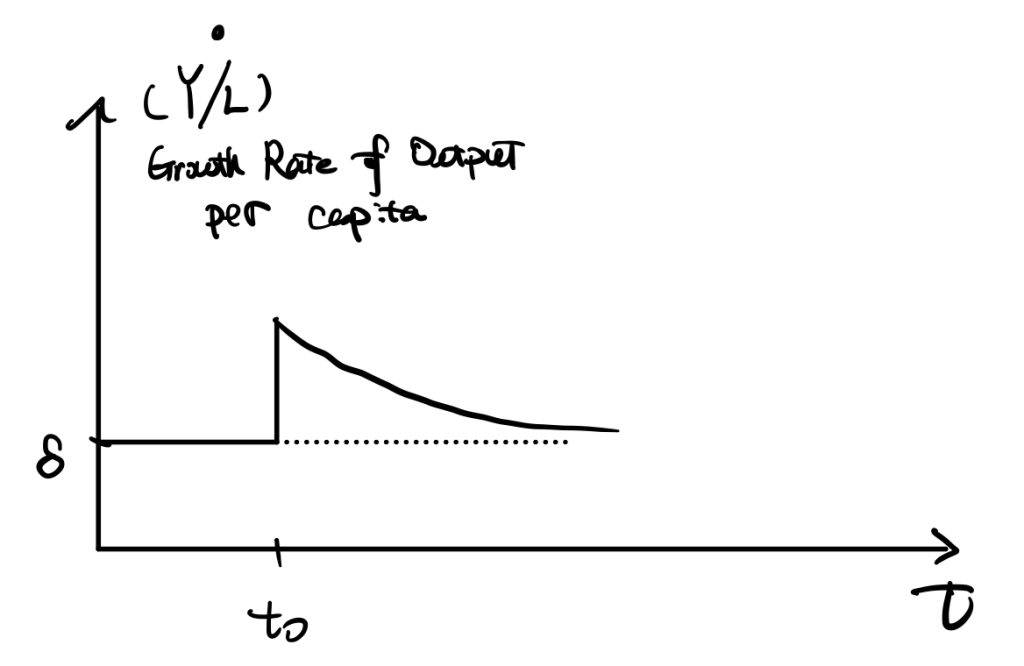
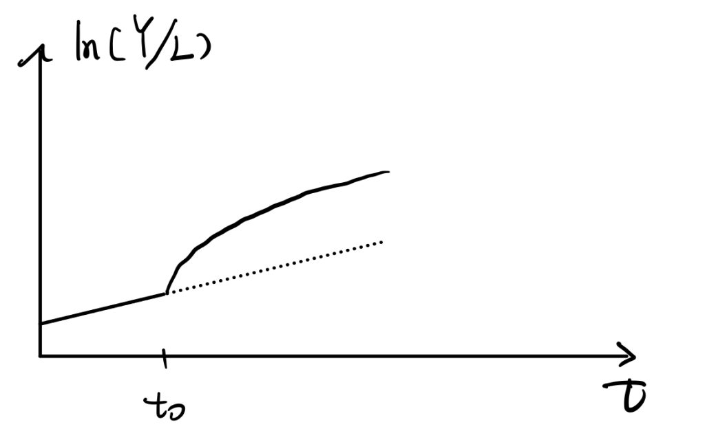
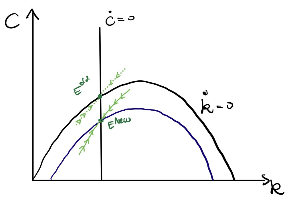
\(\rho\) Changes

A fall in \(\rho\) can be considered as the effect of monetary policy. A fall in \(\rho\) would result in a movement of \(\dot{c}=0\) curve to the right by the equality, \(\frac{\dot{c}}{c}= \frac{r(t)-\rho-\theta g}{\theta} =\frac{f'(k)-\rho-\theta g}{\theta}\).

P.S. \(\dot{c}=0 \Leftrightarrow f'(k)=\rho-\theta g \to k=f’^{-1}( \rho-\theta g )\)

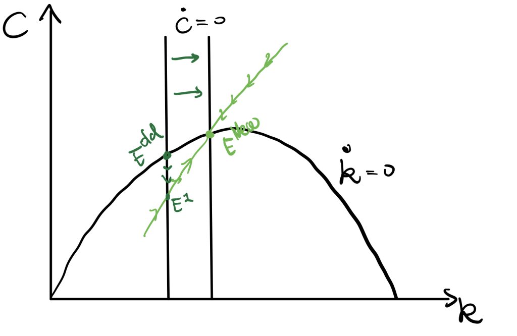
As \(\rho\) changes, a new path generates. The economy is at \(E^1\), and then follows the new path moving to \(E^{new}\). We would finally end up with a new equilibrium with higher consumption.

Convergence

See Romer (2018) find the speed of adjustment.

Recall two paths in the R.C.K model.

$$ \dot{k}=f(k(t))-c(t)-(n+g)k(t) $$

$$ \frac{\dot{c}}{c}=\frac{f'(k)-\rho-\theta g}{\theta} $$

We replace this non-linear equation with the linear approximation, so we take the first order Taylor approximation around the equilibrium \(k^*\) and \(c^*\).

$$ \dot{k} _{approx} \approx \dot{k}|_{k^*,c^*}+\frac{\partial \dot{k}}{\partial k}|_{ k^*,c^* }(k-k^*) \\+ \frac{\partial \dot{k}}{\partial c}|_{ k^*,c^* }(c-c^*) $$

As in the equilibrium \( \dot{k}|_{ k^*,c^* } =0\) and \( \dot{k}|_{ k^*,c^* }=0 \), so

$$ \dot{k}_{approx}\approx \frac{\partial \dot{k}}{\partial k}|_{ k^*,c^* }(k-k^*)+\frac{\partial \dot{k}}{\partial c}|_{ k^*,c^* }(c-c^*) $$

Similarly, (after we doing a bit transformation \( \dot{c}=\frac{f'(k)-\rho-\theta g}{\theta}c \) ).

$$ \dot{c} _{approx} \approx \frac{\partial \dot{c}}{\partial k}|_{ k^*,c^* }(k-k^*)+\frac{\partial \dot{c}}{\partial c}|_{ k^*,c^* }(c-c^*) $$

We then replace \( \dot{c}=\frac{f'(k)-\rho-\theta g}{\theta}c \) ) and \( \dot{k}=f(k(t))-c(t)-(n+g)k(t) \) into \( \dot{k}_{approx} \) and \( \dot{c}_{approx} \). Also, we denote \(\tilde{c}=c-c^*\) and \(\tilde{k}=k-k^*\).

P.S. \(\partial \frac{\dot{c}}{\partial k}|_{ k^*,c^* }=\frac{c^*}{\theta}f”(k^*)\) and \(\frac{\partial \dot{c}}{\partial c}|_{ k^*,c^* }= \frac{f'(k)-\rho-\theta g}{\theta} |_{ k^*,c^* }=\frac{\dot{c}}{c}|_{ k^*,c^* }=0\).

And, \(\frac{\partial \dot{k}}{\partial k}|_{ k^*,c^* }=f'(k^*)-(\delta+n) \) and \(\frac{\partial \dot{k}}{\partial c}|_{ k^*,c^* }=-1\).

Then, we get,

$$ \dot{k}_{approx}\approx [f'(k^*)-(\delta+n)] \tilde{k}-\tilde{c} $$

In equilibrium, \(\dot{c}=0 \Leftrightarrow f'(k)=\rho+\theta g\), so,

$$ \dot{k}_{approx}\approx [\rho+\theta g-(\delta+n)] \tilde{k}-\tilde{c} =\beta \tilde{k}-\tilde{c} $$

$$ \dot{c} _{approx} \approx \frac{c^* f”(k^*)}{\theta } \tilde{k}$$

Then, we divide both side by \(tilde{k}\) or \(\tilde{c}\), respectively. We would get,

$$ \frac{\dot{k}_{approx}}{\tilde{k}}\approx \beta -\frac{\tilde{c}}{\tilde{k}} $$

$$ \frac{\dot{c} _{approx}}{\tilde{c}} \approx \frac{c^* f”(k^*)}{\theta } \frac{\tilde{k}}{\tilde{c}} $$

From the above two equations we can find growth rate of \(\dot{\tilde{c}}_{approx}\) and \( \dot{\tilde{k}}_{approx} \) depend only on the ratio, \(\frac{\tilde{k}}{\tilde{c}}\).

Later, we apply a very strong assumption that \(\tilde{c}\) and \(\tilde{k}\) changes at the same rate, and also the rate make LHS of two equations equal. By this assumption, we denote,

$$ \frac{\dot{c} _{approx}}{\tilde{c}}= \frac{\dot{k}_{approx}}{\tilde{k}} =\mu $$

Then, solving those three equations by making above two equations equal, we would get,

$$\mu^2-\beta \mu +\frac{ f”(k^*) c^* }{\theta}=0$$

$$\mu_1,\mu_2=\frac{\beta\pm[\beta^2-4f”(k^8)c^*/\theta]^{1/2}}{2}$$

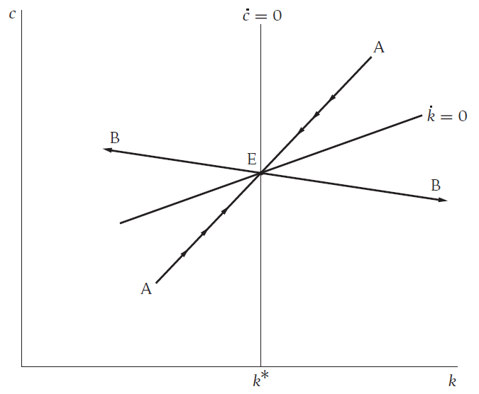
We can see \(\mu\) must be negative, otherwise the economy cannot converge (see the path BB). If \(\mu<0\), the economy would be in the path AA instead. The path is the saddle path of R.C.K. model.

Applying such as the Cobb-Douglas form production, we can plug second derivatives of the production into \(\mu\) and get the speed of adjustment.

Based on many years of study of the Solow model, I learned different versions of it. Although all of them are talking about the same theory, there are some differences in the learning structure and functional forms of the model. Now, I revisit the Solow model mainly based on the original paper (Solow, 1956). Here is a summary of the Solow model.

Robert Solow was awarded the Nobel Prize in 1987 for his contributions to the theory of Economic Growth.

Start

All theory depends on assumptions which are not quite true. That is what makes it theory. The art of successful theorizing is to make the inevitable simplifying assumptions in such a way that the final results are not very sensitive. 1 A “crucial” assumption is one on which the conclusions do depend sensitively, and it is important that crucial assumptions be reasonably realistic. When the results of a theory seem to flow specifically from a special crucial assumption, then if the assumption is dubious, the results are suspect.

The above paragraph is the beginning of his paper. That is the first time I read this paper. It really shocks me and brings me a different understanding about economic theory.

Assumption

1. Only one commodity, output as a whole. \(Y(t)\), by which output equals income.
2. For each agent, \(Y(t)=consumption+saving/investing\). That is equivalent to assuming no government and net export, \(Y=C+I+G+NX\).
3. Net investment equals saving. (1) \(\frac{\partial K}{\partial t}=\dot{K}=s\cdot Y(t)\).
4. Output is produced by two factors, labour and capital. (2) \(Y=F(K,L)\). Also, the production function is homogenous of degree one and CRTS.

Solve

Insert (1) into (2), we would get

(3)\(\quad \dot{K}=sF(K,L) \)

As \(s\) is exogenous, thus (3) has two unknowns, so it is unable to be solved. To solve (3), we need to know something about labour.

There are mainly two ways of finding labour. Way 1: \(MPL=\frac{W}{P}\), which is the marginal productivity of labour equals real wage rate. Then, we can solve the labour supply. Way 2: take a general form. Making labour supply \(=f(W/P\). In any case, there are three unknowns, \(W,P,\) and \(L\).

However, we here assume an exogenous population growth rate \(n\). Thus,

(4) \(\quad L(t)=L_0\cdot e^{nt} \)

(easy to show \(ln(\frac{L_t}{L_{t-1}})=n\) and \(\frac{\dot{L_t}}{L_t}=n\).)

This term can be considered as the labour supply. It says that an exponentially growing labour force is offered. Employment is completely inelastic.

Put (4) into (3), we would get,

(5) \(\dot{K}=sF(K,L_0e^{nt})\).

, which is the time-path of capital accumulation under full employment.

(5) is a differential equation, and \(K(t)\) is the only variable. The solution could tell us, (all the followings are under full employment)

1. the time path of capital.
2. \(MPL=w\), and \(MPK=r\). The time-path of real wage rate and capital rent rate.
3. By given saving rate, we would also know saving and consumptions.

We introduce a new variable\(k=\frac{K}{L}\), which is capital per capita.

Thus, \(K=kL=kL_0e^{nt}\). The, differentiate w.r.t. \(t\), we get,

$$\dot{K}=\dot{k}L+K\dot{L}=\dot{k}L_0e^{nt}+nkL_0e^{nt}$$

Combining with (5),

$$ \dot{k}L_0e^{nt}+nkL_0e^{nt}=sF(K,L_0e^{nt}) $$

$$ \dot{k}=sF(k,1)-nk $$

Graphically, (r is k in my definition).

Easy to see that if the production function is increasing and diminishing and shaped as the figure above, then the interaction \(k^*\) would be a stable value (easy to show by discussing before \(k^*\) and after. e.g. if before k* then \(\dot{k}>0\), there is the accumulation of capital per capita).

Some simple math,

$$k=\frac{K}{L}$$

$$ ln(k)=ln(K)-ln(L) $$

Differentiate w.r.t. \(t\),

$$ \frac{\dot{k}}{k}= \frac{\dot{K}}{K}- \underbrace{\frac{\dot{L}}{L}}_{n} $$

When\( \frac{\dot{k}}{k} =0\), then \( \frac{\dot{K}}{K} = \frac{\dot{L}}{L}=n\). The implication is that at \(k^*\) (two lines interact, and make \( \frac{\dot{k}}{k} =0\) ) the time-path of labour equal that of capital.

In addition, for Y and y,

$$ln(Y)=ln(F(K,L))$$

Differentiate w.r.t. \(t\),

$$ \frac{\dot{Y}}{Y}=\frac{ \dot{K}F_1’+\dot{L}F_2′ }{F(K,L)} $$

By Euler’s Theorem (see math tools),

$$ \frac{\dot{Y}}{Y}=\frac{ \dot{K}F_1’+\dot{L}F_2′ }{KF’_1+LF’_2}=\frac{ \frac{\dot{K}}{KL}F’_1 +\frac{\dot{L}}{KL}F’_2}{\frac{F’_1}{L}+\frac{F’_2}{K}} $$

\frac{\dot{Y}}{Y}=\frac{ \dot{K}F_1’+\dot{L}F_2′ }{KF’_1+LF’_2}=\frac{ \frac{\dot{K}}{KL}F’_1 +\frac{\dot{L}}{KL}F’_2}{\frac{F’_1}{L}+\frac{F’_2}{K}}

\frac{\dot{Y}}{Y}= \frac{ \frac{\dot{K}}{K}\frac{F’_1}{L} +\frac{\dot{L}}{L}\frac{F’_2}{K}}{\frac{F’_1}{L}+\frac{F’_2}{K}}= \frac{n\times ( \frac{F’_1}{L}+\frac{F’_2}{K} )}{ \frac{F’_1}{L}+\frac{F’_2}{K} }

$$ \frac{\dot{Y}}{Y}=n $$

$$ y=\frac{Y}{L} $$

$$ ln(y)=ln(Y)-ln(L) $$

$$ \frac{\dot{y}}{y}= \frac{\dot{Y}}{Y}- \frac{\dot{L}}{L}=n-n=0 $$

The introduction of Solow (1956) ends there (there are analysis of applying different functional forms of production in his paper, but I would not discuss here), the following are a summary of my previous learning.

P.S. there is no depreciation in the original Solow model.

In summary, the key assumptions are: 1, the law of motion of capital accumulation \(\dot{K}=I\); 2, the shape of the production function.

Solow followed this paper with another pioneering artical, “Technical Change and the Aggregate Production Function.” Before it was published, economists had believed that capital and labour were the main causes of economic growth. But Solow showed that half of economic growth cannot be accounted for by increases in capital and labour.This unaccounted-for portion of economic growth—now called the “Solow residual”—he attributed to technological innovation.

Reference

Solow, 1956

Robert Merton Solow