Quantity Theory of Money (QTM)

My current reviews of how the aggregate demand curve is determined and how is the development of Keynesianism and Monetarism encourage me to get further insights into QTM, which is also one of the oldest and currently surviving economic theory.

Karl Marx

Let’s begin the story with Karl Marx who is not the pioneer of QTM but partially believed it. His idea about money is that the amount of money in circulation is determined by the quantity of goods times the prices of goods.

Keynes

John Maynard Keynes also agreed on part of the QTM, but he held a different opinion about the determinant of the quantity of money. He thought that the amount of money depends on the purchasing power or aggregate demand.

Keynes also thought output and velocity (k) is not stable in the short run. (coincide with his idea of price is super sticky in the very short run)

The Cambridge equation formed as the following,

\( M^d=k \cdot P \cdot Y \)

Alfred Marshall, A.C. Pigou, and John Maynard Keynes assumed that money demand is determined by \(k\), which represents a percentage of money hoarded in hands, times the nominal income \( P\cdot Y\).

P.S. Dr. Rendahl at Cambridge taught that part in S201 Applied Macroeconomics before, but I did not get it when I am as a student. Liquidity traps would be introduced in a later blog.

Friedman

Friedman held the similar idea with Keynes that the velocity would not fixed in the short run. He also stated that the velocity might not offset the effect of money growth, instead velocity moves in the same direction and reinforece with money growth empircally. For example, when quantity of money increase, the velocity rises as well (p.s. my idea: is that still true during the covid crisis? The U.S. example might not be the case, but needs data to prove).

In summary, Marx, Keynes, and Friedman all agreed with the quantity theory of money, but they have different ideas. Marx emphasised the productions, Keynes the demand and income, and Friedman the supply or quantity of money.

Empircal Study

Here are a maths and empircal studies.

\( M\cdot V=P\cdot Y \)

In the long run, velocity and real output are constant, so money supply is positively correlated with the price level. However, in the short run, the output is not fixed, so changes in the money supply would change the real output.

By log transformation,

\( m+v=p+y \)

\( v=p+y-m \)

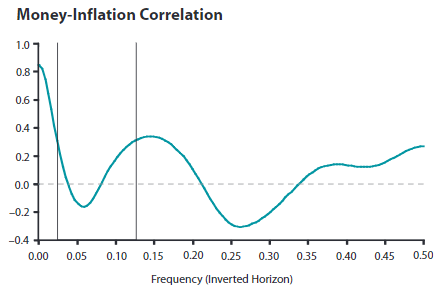
So the changes in velocity are determined by three parts, inflation, real output growth, and money growth. As shown in the figure below, some emprical data tell that correlation between money growth and inflation (y-axis) is close to one, about 0.82 exactly (as frequency is close to 0, means infinite long time period). Where the frequency (x-axis) means the frequency of periods used into the study. 0.5 frequency means horizon of changes in 2 periods (one period is a quarter as data are quarterly recorded). This study tells that in the long run, inflation is correlated with money growth, but the correlation is not that clear in the short run.

Ideas

1. By the Cambridge method, quantity of money is determined by people’s income times a portion \(k\), and that \(k\) would definitely changable with the macroeconomic condition. For example, in the recession, people are more likely to hoard more money for security reason, even interest rate is close to zero by liquidity trap. How that \(k\) is determined, orhow to meature it? Also, how government and central banks’ policy could change people’s willingness of holding money?

Reference

Marx, K., 1911. A contribution to the critique of political economy. CH Kerr.

Wen, Y., 2002. The business cycle effects of Christmas. Journal of Monetary Economics, 49(6), pp.1289-1314.

Wen, Y., 2006. The quantity theory of money. Monetary Trends, (Nov).