1. Perceptron
1.1 AND & OR & ‘N’ Gate
Linear Classification might be applied by AND & OR.
import numpy as np

def AND(x1, x2):
    x = np.array([x1,x2])
    w = np.array([0.5, 0.5])
    b = -0.7
    temp = np.sum(w*x )+ b
    if temp<= 0:
        return 0
    else:
        return 1

def NAND(x1,x2):
    x = np.array([x1, x2])
    w = np.array([-0.5, -0.5])
    b = 0.7
    temp = np.sum(w*x)+b
    if temp <= 0:
        return 0
    else:
        return 1

def Nand(x1, x2): # same as above
    return int(not bool(AND(x1,x2)))


def OR(x1,x2):
    x = np.array([x1, x2])
    w = np.array([0.5, 0.5])
    b = -0.2
    temp = np.sum(w*x) + b
    if temp <=0:
        return 0
    else:
        return 1
1.2 XOR Gate – Apply More than Two Perceptrons to Achieve Non-Linear Classification


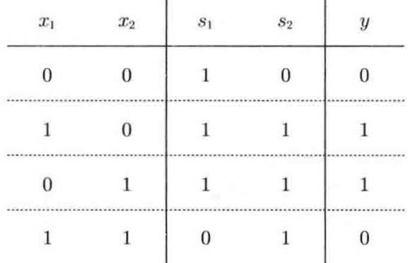
def XOR(x1, x2):
    s1 = NAND(x1, x2)
    s2 = OR(x1,x2)
    y = AND(s1, s2)
return y- It has been proved that any functions could be represented by a combination of 2 perceptrons with sigmoid as the activation function.
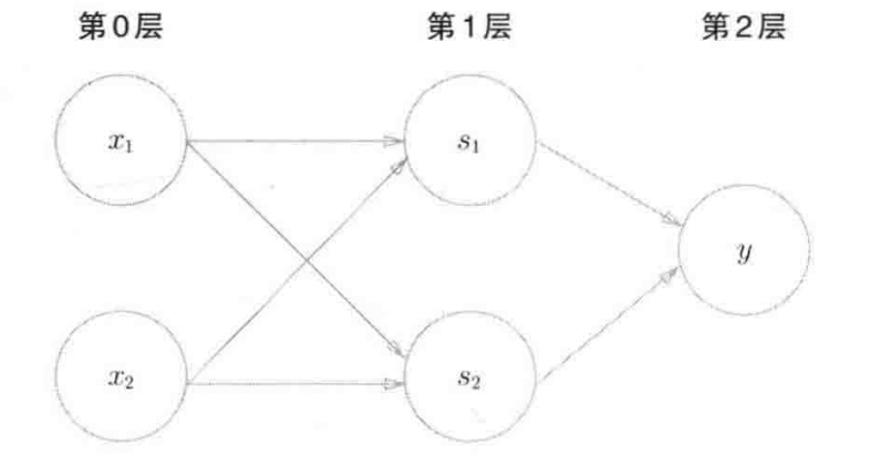
Apply Multi – Layers of Perceptrons, we can achieve the simulation of any non-linear transformation. An important part is that Activation Function is necessary to be inserted into different layers. It can be easily proved that:
$$ W_2\Bigg( \big(W_1 X + b_1 \big) \Bigg) + b_2 \equiv W^* x + b^*$$
Multi-layer of Linear Transformation is still Linear Transformation. So, multi-layer of perceptrons becomes useless without Activation Function.
However, if activation function, in other word a non-linear transformation, is added between layers, then the neural network could mimic any non-linear function.
- Therefore, what the Deep Learning is doing is to apply multi-layer perceptrons to mimic the pattern of a certain thing. Some key points are
- (1) multi-layer perceptrons are named the Neural Network. Each adjacent layers are doing linear transformation WX + b and then apply a activation function, such as Sigmoid(x) = \frac{1}{1+e^{-x}};
- (2) Update the weight matrix W and b, until the neural network could output an “optimal” result.
- (1) How to define the layers and network structure, (2) how to evaluate the result is “Optimal” or not, and (3) how to find the weights are the main problems in Deep Learning.
2. Network Structure – Forward Propagation
Let’s start with the first Question. How to define the layers and network structure. Through the Network,
- we input Data, X, initially.
- Data are transformed by ( Perceptrons – “Affine”, Activation Functions ) multi-times, which are the multi-layers.
- Then, the results are passed through a Softmax function to reform results into percentages.
- Finally, a Loss is calculate.
$$ x \to f(.) \to a(.) \to \text{…} \to Softmax(.) \to Loss(.)$$
, where f(x) = xw + b
, where a(x) is the activation function.
, where Loss(x) is the loss function.
2.1 Affine – Linear Transformation

$$ f(X) = X \cdot W +b $$
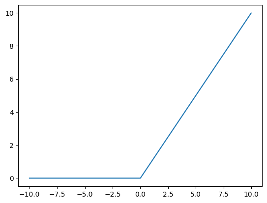
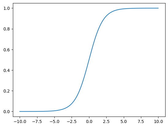
2.2 Activation Function
- ReLU, f(x) = max(x, 0
- Sigmoid, f(x) = \frac{1}{1+e^{-x}}
- tanh
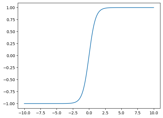
There are some properties of activation function, such as symmetric to the zero point, differentiable, etc. Those details are not discuss here.
2.3 Softmax
$$ \vec{X} = (x_1, …, x_i, ..) $$
$$ Softmax(\vec{X}) = \vec{Y} = (…, \frac{e^{x_i}}{\sum e^{x_i}} ,…)^T $$
Inputs are reform to be percentages, and those percentages are sum to be one.
P.S.
$$ y_k = \frac{e^{a_k}}{\sum_{i=1}^{n}e^{a_i} } = \frac{C e^{a_k}}{C \sum_{i=1}^{n}e^{a_i} } $$
$$ = \frac{e^{a_k+ lnC} }{\sum_{i=1}^{n}e^{a_i + lnC} } $$
$$ = \frac{e^{a_k – C’} }{\sum_{i=1}^{n}e^{a_i – C’} } $$
为了防止溢出,事先把x减去最大值。最大值是有效数据,其他值溢不溢出可管不了,也不关心。
2.4 Loss Function
- Cross Entropy, L = -\sum t_i \ ln(y_i) = – ln(\vec{Y}) \cdot \mathbf{t}^T
- MSE, See “Linear Regression Paddle” note. E = \frac{1}{2} \sum_k (y_k – t_k)^2
3. Minimise Loss & Update Weights
We consider the “Optimal” weights are such that they can result in minimum loss. So, in other words, we aim to find w and b that can minimise the loss function.
How to Do It ?
$$ arg\min_{w, b} Loss $$
$$ \hat{w}: \frac{\partial L}{\partial w} = 0 ,\quad \hat{b}: \frac{\partial L}{\partial b} = 0$$
Remember, the pathway:
$$ x \to f(.) \to a(.) \to \text{…} \to Softmax(.) \to Loss(.)$$
To solve the `F.O.C, we need to apply the Chain rule backward, which is called the Backward Propagation.
By Chain Rule,
$$ \frac{\partial Loss(w)}{\partial w} = \frac{\partial Loss(.)}{\partial Softmax} \cdot \frac{\partial Softmax(.)}{\partial a} \cdot \frac{\partial a}{\partial f} \cdot \frac{\partial f}{\partial a} … \cdot \frac{\partial f}{\partial w} $$
Let’s Decompose each Part in the Following.
3.1 Loss
$$ \frac{\partial Loss(\vec{Y}, \vec{t})}{\partial \vec{Y}} $$
- Cross Entropy
$$ L = -\sum t_i \ ln(y_i) = – ln(\vec{Y}) \cdot \mathbf{t}^T$$
$$\frac{\partial L}{\partial y_i} = – \frac{t_i}{y_i}$$
$$\frac{\partial L}{\partial \vec{Y}} = – \big(…,\frac{t_i}{y_i},…\big)^T$$
3.2 Softmax
$$ \vec{X} = (x_1, …, x_i, ..) $$
$$ Softmax(\vec{X}) = \vec{Y} = (…, \frac{e^{x_i}}{\sum e^{x_i}} ,…)^T $$
$$ \frac{\partial Softmax(\vec{X})}{\partial \vec{X}} = Diag(\vec{Y}) – Y\cdot Y^T $$
Deviation is as the Following,
https://blog.csdn.net/Wild_Young/article/details/121912675
$\frac{\partial Y}{\partial X}$:
$$Softmax(x) = \frac{1}{1+e^{-x}}$$
Let X be a vector with shape = (n,1), and
$Y = Softmax(X) $.
That means, for each element of y_i in Y
$$ y_k = \frac{-e^{x_k}}{\sum_i^N e^{x_i}} $$
So,
$$ \frac{\partial Y}{\partial x_k} $$
If j = i,
$$ \frac{\partial y_j}{\partial x_i} = \frac{\partial }{\partial x_i} \Bigg( \frac{e^{x_i}}{\sum e^{x_i}} \Bigg) $$
$$ = \frac{ (e^{x_i})’\sum e^{x_i} – e^{x_i} (\sum e^{x_i})’ }{\big( \sum e^{x_i} \big)^2} $$
$$ =\frac{e^{x_i}}{\sum e^{x_i}} – \frac{e^{x_i}}{\sum e^{x_i}} \cdot \frac{e^{x_i}}{\sum e^{x_i}}$$
$$= y_i – y_i^2 =y_i(1-y_i)$$
If j \neq i,
$$ \frac{\partial y_j}{\partial x_i} = \frac{\partial }{\partial x_i} \Bigg( \frac{e^{x_j}}{\sum e^{x_i}} \Bigg) $$
$$ = \frac{-e^{x_i} e^{x_j}}{(\sum e^{x_i})^2} $$
$$ =- \frac{e^{x_j}}{\sum e^{x_i}} \cdot \frac{e^{x_i}}{\sum e^{x_i}} $$
$$ = -y_j y_i $$
$$ \frac{\partial y_j}{\partial x_i}=y_i – y_i^2 \quad \text{,if $i = j$} $$
$$\frac{\partial y_j}{\partial x_i} = -y_j y_i \quad \text{,if $i \neq j$} $$
Therefore, for \frac{\partial Y}{\partial X}, we got the Jacobian matrix,
$$\frac{\partial \vec{Y}}{\partial \vec{X}} = Diag(Y) – Y^T Y$$
However, in the backward propagation of Softmax, we only need the diagonal, which is in the case of i = j.
$$ \frac{\partial y_i}{\partial x_i} = y_i-y_i^2 =y_i(1-y_i)$$
3.3 Loss (Cross-Entropy) and Softmax
There is a trick with the combination between cross-entropy-error and softmax.
The Cross-Entropy Loss function is,

, where \vec{Y_{log}}^T is apply log to each element of \vec{Y}, and then take transformation.
https://www.matrixcalculus.org
$$\frac{\partial L}{\partial \vec{Y}} = \vec{\mathbf{t}}^T \cdot Diag(Y_{1/Y}) $$
, where Y_{1/Y} is 1/y_i for each element of Y.
$$ \frac{\partial L}{\partial x_k } = \frac{\partial L}{\partial y_k}\cdot \frac{\partial y_k}{\partial x_k} $$
$$\frac{\partial L}{\partial x_k } =- \sum_i \frac{\partial }{\partial {y}_k} \bigg( t_i \ ln(y_i) \bigg) \cdot \frac{\partial y_k}{\partial x_k} $$
$$\frac{\partial L}{\partial x_k } =- \sum_i \frac{t_i }{{ y}_i} \cdot \frac{\partial {y}_i}{\partial x_k} $$
Plug in the derivatives of Softmax, \frac{\partial y}{\partial x}
$$\frac{\partial L}{\partial x_k } = – \frac{t_k }{{ y}_k}
\cdot \frac{\partial {y}_k}{\partial x_k} \sum_{i\neq k} \frac{t_i }{{ y}_i} \cdot \frac{\partial {y}_i}{\partial x_k} $$
$$ = -\frac{t_k }{{ y}_k}
\cdot {y}_k (1-{y}_k) \sum_{i\neq k} \frac{t_i }{{ y}_i} \cdot (- {y}_i {y}_k)
$$
$$ = – t_k (1-{y}_k) \sum_{i\neq k} t_i {y}_k
$$
$$ = – t_k \sum_{i} t_i \ {y}_k
$$
$$ = – t_k {y}k \sum{i} t_i \quad\text{by the tag, $t$, is sum to be 1}
$$
$$ \frac{\partial L}{\partial x_k } ={y}_k – t_k$$
So, we get \frac{\partial L}{\partial x_k} ={y}_k – t_k.
3.4 Affine
$$ \frac{\partial f}{\partial w} $$
$$ \frac{\partial f}{\partial b} $$
- Backward
$$ \frac{\partial f}{\partial X} =\cdot \ W^T \quad \text{, Right Multiplied}$$
$$ \frac{\partial f}{\partial W} = X^T \cdot \ \quad \text{, Left Multiplied}$$
$$ \frac{\partial f}{\partial b} = \mathbf{1}^T \cdot \quad \text{, Left Multiplied} $$
4. Other Theoretical Details
- Batch: mini-batch and epoch for improving training accuracy.
- Weights Initialisation: Xavier – Sigmoid and tank, He – ReLU
- Weights Updating: SGD, Momentum, Adam, etc.
- Overfitting: Batches, Regularisation, Dropout.
- Hyperparameters: Bayes
See Chapter 6 of the book.
5. Code
See Attachment for the Code Realisation by purely Numpy.
Code and Books: http://82.157.170.111:1011/s/9D9BCBbCop6ERaD
One thought on “Deep Learning from Scratch”
Comments are closed.