Optimiser

In the Neural Network, we optimise (minimise) the loss by choosing weights matrix, $W$ and $b$.

$$arg\underset{W,b}{max}Loss$$

By taking the F.O.C., we get the gradient, $\nabla$. Then, we update weights by minus the learning rate times the gradient.

Here, I wrote some test algorithms to find how optimisers evolve.

Preparation

Let’s make some preparations and notation clarifications.

Notation:

• Y is True,
• T is the Estimate.

$$Y=XW+b+e$$

Let $T = WX +b$

$$loss=e^{T}e$$

$$loss=(Y-T{)}^T\cdot (Y-T)$$

$$=(WX+b+e-T{)}^T\cdot (WX+b+e-T)$$

$$\frac{\partial Loss}{\partial W}=X^T(WX+b+e-T)=2X^T(Y-T)$$

$$\frac{\partial loss}{\partial b}=1^T(WX+b+e-T)=1^T(Y-T)$$

Just One More Thing We Consider Here!

We do not want the number of sample to affect loss function’s value, so we take averge, instead of sumation.

$$\frac{\partial Loss}{\partial W}=\frac{2}{N}{X}^T(Y-T),\frac{\partial loss}{\partial b}=\frac{1}{N}{1}^T(Y-T)$$

Optimisers

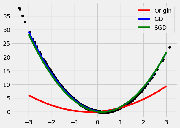
Gradient Descent

$$W_t=W_{t-1}–\eta {\mathrm{\nabla }}_W$$

$$b_t=b_{t-1}–\eta {\mathrm{\nabla }}_b$$

, where $\eta$ is the learning rate.

However, we may find that the Gradient Descent might not satisfactory, because gradients might not be available or vanished sometimes. Also, the process of gradient descent largely depends on the HyperParameter $\eta$. Some other methods of optimisation are developed.

Different Optimisers aim to find the optimal weights more speedy and more accurate. In the followings are how optimisers are designed.

Stochastic Gradient Descent – SGD

In SGD, the stochastic part is added to avoid model train full dataset, and avoid resulting in the problem of overfitting.

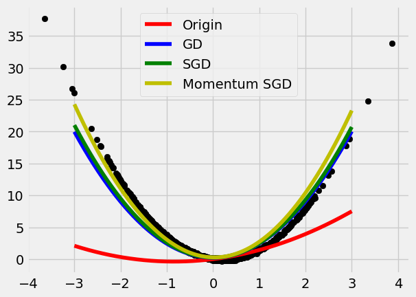
Momentum SGD

A momentum term is added.

• Apply Momentum to the Gradient, $\nabla$.

$$\text{Gradient Descent:}{w}_t=w_{t-1}-\eta g_w$$

$$\text{Momentum:}{v}_t={\beta }_1{v}_{t-1}+(1-{\beta }_1)g_w$$

In the Beginning of Iteration, $v_0=0$, so we amend it to be $\hat{v_T}$

$$\widehat{v_t}=\frac{v_t}{1-{\beta }_1^t}$$

,where $\beta_1$ assign weights between previous value and the gradient.

Replace the gradient $g_w$ by the amended momentum term $\hat{v}_t$:

$$w_t=w_{t-1}-\eta {\hat{v}}_t$$

P.S. Why we amend $v_t$ by dividing $1 + \beta^t$.

As $v_t = \beta_1 v_{t-1} + (1-\beta_1)g_w$, which is like a geometric decaying polynomial function. The difference is that $w$ and $g_w$ keep updating each period. Let’s assume there is no updating anymore, or in other word, model has converge. $g_w = constant$. $\{ v_t \}_{t=0}^T$ would be,

$$v_0=0$$

$$v_1=(1-{\beta }_1)g_w$$

$$v_2={\beta }_1(1-{\beta }_1)g_w+(1-{\beta }_1)g_w$$

$$v_3={\beta }_1^2(1-{\beta }_1)g_w+{\beta }_1(1-{\beta }_1)g_w+(1-{\beta }_1)g_w$$

$$v_n={\beta }_1^{n-1}(1-{\beta }_1)g_w+\dots +(1-{\beta }_1)g_w$$

$$v_n=(1-{\beta }_1)g_w(1+{\beta }_1+\dots +{\beta }_1^{n-1})$$

$$v_n=(1-{\beta }_1)g_w\frac{1–{\beta }_1^n}{1-{\beta }_1}=g_w(1-{\beta }_1^n)$$

Clearly, to amend $v_n$ be like $g_w$, we need to divide it by $1-\beta_1^n$, because of the polynomial ‘geometric’ form.

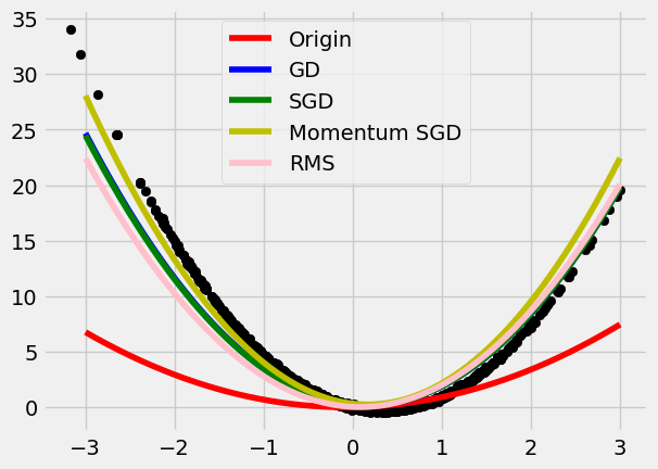
RMSprop

• Apply a Transformation to the Gradient, $\nabla$.

$$\text{Gradient Descent:}{w}_t=w_{t-1}-\eta g_w$$

$$\text{RMS:}{m}_t={\beta }_1{v}_{t-1}+(1-{\beta }_2)g_w^2$$

In the Beginning of Iteration, $v_0=0$, so we amend it to be $\hat{v_T}$, (remember there is a power $t$ here).

$$\widehat{m_t}=\frac{m_t}{1-{\beta }_1^t}$$

,where $\beta_1$ assign weights between previous value and the gradient.

Add a square root of $\hat{m}_t$ in the denominator:

$$w_t=w_{t-1}-\eta \frac{g_w}{\sqrt{{\hat{m}}_t}}$$

Adam

Adam is nearly the most powerful optimiser so far. Adam is like a combination of Momentum and RMS, both $\hat{m}$ and $\hat{v}$ are added to adjust the speed of approaching to the optimal points, $W^*$, and $b^*$.

$$w_t=w_{t-1}–\eta \cdot \frac{{\hat{v}}_t}{\sqrt{{\hat{m}}_t}}$$

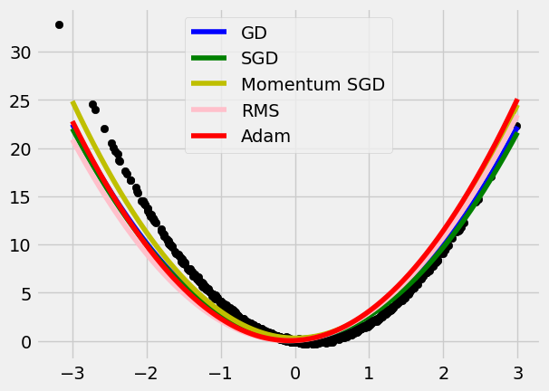
Three main hyper parameters are $\eta = 0.01$, $\beta_1 = 0.9$, and $\beta_2 = 0.999$.

Code