Fanyu Zhao

Four potential solutions,

1. Covential Monetary policy
2. Forward guidance
3. Internal devaluations
4. Quantitative easing

Covential Monetary policy

Recall the public sectors budget constraint is ,

$$ G_t-d_{t+1}=T_t+(m_t-m_{t-1})-(1+i_t)d_t $$

or

$$ \underbrace{G_t+(1+i_t)d_t}_{Money Spending}=\underbrace{T_t+(m_t-m_{t-1})+d_{t+1}}_{Money Source} $$

In a standard open market operation, \(d_{t+1}\) (and \(b_{t+1}\)) would fall, and \(m_t-m_{t-1}\) would rise by the same amount. CB or Gov buy back debts and pool money into the market, so the net debt outstanding decrease and amount of money oustanding increase.

$$ G_t+(1+i_t)d_t=T_t+(\uparrow m_t-m_{t-1})+\downarrow d_{t+1} $$

Or through helicopter drop, reducing tax \(T_t\) to increase \(m_t-m_{t-1}\) .

$$ G_t+(1+i_t)d_t=\downarrow T_t+(\uparrow m_t-m_{t-1})+ d_{t+1} $$

How private sectors react to the windfall of money?

Assume in advance that there is a reversal of monetary injection in the period \(t+1\).

$$ u'(\hat{y})=\beta \frac{\bar{p}_t}{m_{t+1}}y’u'(y’) $$

Nothing really changes in the Euler equation for private sectors. In other words, \( \hat{y} \) is still decresed from \(y_t\), and is not affected by changes in \(m_t\). \(p_t=\frac{m_t}{y_t}\), partially because \(p_t\) is predetermined already.

Intuitively, private sectors know the money would be taxed back, so they just hold the extra money (hoard them), and will pay them back as future tax payments. (That’s is the way to make the Euler equation hold). The excess cash holding would not bring an increase in future consumption, because that cash is all for future taxes. Consider the Ricardian Equilibrium.

P.S. that could be a Pareto-improvement to coordinate on spending.

As Keynes called “Pushing on a string”. Even if CB drops money from helicopters, the money would not be spent and would be hoarded. Therefore, no real impacts on the economy.

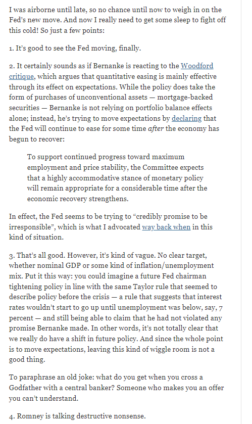
As shown in the figure, an increase in the money supply (monetary base) would result in people holding more money (excess reserve). At the moment in around 2008, the effective federal fund rate hits zero, liquidity traps started. Injecting more money (increasing the money supply) cause excess cash holding, instead of current output increase.

Forward Guidance

Forward guidance means committing to change things in the future (, with perfect credibility).

Assume that he government commits to expand money supply from /(m/) to /(m’/) in period \(t+1\) onward. Also, assume not in the liquidity trap in \(t+1\), (\(v_{t+1}=1\)). So the price level at \(t+1\) would be,

$$ p_{t+1}=\frac{m’}{y’}>\frac{m}{y’} $$

The Euler equation,

$$ u'(y_t)=\beta \frac{p_t}{p_{t+1}}u'(y’) $$

now becomes,

$$ u'(y_t)=\beta \frac{\bar{p}_t}{m_{t+1}}y’u'(y’) $$

And \(m_{t+1}\) is increased to \(m’\), so

$$ u'(y_t)=\beta \frac{\bar{p}_t}{m’}y’u'(y’) $$

An estimated decrease in future outputs would increase \(y’u'(y’)\). However, a permanent increase in \(m’\) to keep the equation unchanged.

Forward Guidance differs from the conventional monetary policy because an extra amount of money would not be taxed back. The central bank “commits to act irresponsibly” in the future. Also, the conventional monetary policy emphasises the current money supply, but forward guidance states the future. People will know that there is no need to pay extra tax back in the future.

The is no clear downward trend of the real output while increasing money supply after getting into the liquidity trap. The market in the US implies that public sectors react to the expected decrease in future output by increasing the money supply in a long period (equivalent to the forward guidance), therefore the real output at the current period does undergo a significant decrease.

See Krugman (1988) and Eggertsson and Woodford (2003).

Internal Devaluations

Here, we consider a production economy instead of an endowment economy. In this way, instead of being endowed with \(y_t\) units of the output good in each period, agents are endowed with one unit of time and they choose an inelastic supply of working.

Firms are perfectly competitive and produce output according to \(y_t=z_t l_t\), where \( z_t\) donates labour productivity and \(l_t\) the amount of labour hired.

A representative firm’s optimisation problem is then given by

$$ \max_{l_t} p_t z_t l_t- \tilde{w_t}l_t $$

F.O.C.

$$p_t z_t =\tilde{w_t} $$

The first-order condition tells that nominal wage stickiness leads to price stickiness. Given wages, \(\tilde{w_t}\), a fall in prices would reduce profits, and firms would shut down their businesses (by perfect competition assumption).

However, if prices and wages fell in equal proportion, firms would still like to hire equally many works. And the fall in prices would boost demand. P.S. the real wages keep constant.

Intuition: Firstly, as prices fall, goods get cheaper. So even 80 of spending can buy100 worth of goods. Secondly, as wages also fall, real profits are unchanged, and firms are willing to meet the additional demand. Finally, the positive impacts on \(y_t\) could offset the negative of it (from underestimated future outputs).

\( \quad \downarrow P \Rightarrow \downarrow W \Rightarrow\) unchanged profits and increase outputs

Quantitative Easing

In the open market operation, the CB purchases short-term government bonds (3-month T-bill). By QE, the CB purchases assets with longer maturity and credibility, see The Fed’s Balance Sheet, e.g. MBS.

The idea of QE is to decrease the interest rate once the short term rate is already zero, and also pool money into the market. In the recession, short term bonds’ nominal interest rates are already zero, but long term bonds may not. Thus, by purchasing long-term bonds, yields are pushed downward (real interest rate falls), and stimulate the economy. (Similar to the non-arbitrage theory). Long-term assets are equally valuable as short term assets at any horizon. In the liquidity trap, short term assets are equally valuable as holding money, so long term assets are perfect subsites to money as well (consider including liquidity premium and risk premium).

In the model with Cash in Advance and short long term assets, we consider include

1. A short term asset (one period) \(b_{t+1}^1\).
2. A long term asset (two periods), \(b_{t+1}^2\).
3. The price of the short-term asset is denoted \(q_t^1\), and pays out one unit of cash in period t+1.
4. The price of the long-term asset is denoted \(q_t^2\), and pays out one unit of cash in period t+2.

The household’s problem is then

$$ \max_{c_t,b^1_{t+1},x_{t+1}} \sum_{t=0}^{\infty} \beta^t u(c_t) $$

$$s.t. \quad q_t^1 b_{t+1}^1+ q_t^2 b_{t+1}^2+x_{t+1}+p_t c_t=b_t^1 +q_t^1 b_t^2 +w_{t-1}+x_t – T_t $$

LHS stands for how to spend money, RHS how money comes from.

F.O.C.

$$ u'(c_t)=\beta \frac{1}{q_t^1} \frac{p_t}{p_{t+1}}u'(c_{t+1}) \quad w.r.t\ b^1$$

$$ u'(c_t)=\beta \frac{q_{t+1}^1}{q_t^2} \frac{p_t}{p_{t+1}}u'(c_{t+1}) \quad w.r.t\ b^2$$

$$ u'(c_t)-\mu_t = \beta \frac{p_t}{p_{t+1}}u'(c_{t+1}) \quad w.r.t\ x$$

Therefore, the finding is,

$$ \beta \underbrace{\frac{q_{t+1}^1}{q_t^2}}_{1+i^2_{t+1}} \frac{p_t}{p_{t+1}}u'(c_{t+1}) = \beta \underbrace{\frac{1}{q_t^1}}_{1+i_{t+1}^1} \frac{p_t}{p_{t+1}}u'(c_{t+1}) = \beta \frac{p_t}{p_{t+1}}u'(c_{t+1}) +\mu $$

Equivalent to \( Return\ of \ LongTerm=Ro\ ShortTerm=Ro\ Cash\).

Long-term bonds are traded at arbitrage with short-term bonds which are traded at arbitrage with money.

Recall that the purpose of QE is to reduce the return on long-term bonds but that cannot be done.

If in the liquidity trap, \( x_{t+1}=0, \mu=0, i_t=0 \Rightarrow \frac{1}{q_t^1}=1 \Leftrightarrow \frac{q_{t+1}^1}{q_t^2}=1 \).

In the figure, the green curve represents QE (Fed Balance sheet). During the 2008 financial crisis and Covid-19, the Fed purchase assets (MBS and Long-term T bonds) and pay with money, in order to release liquidity into the market.

In the end,

1. Convential monetary policy – ineffective
2. Forward guidance – effective
3. Inteernal devaluations – effective but hard
4. Quantitative easing – ineffective