Here, I would use the cash in advance model to illustrate some economic phenomena.
Assumptions
Two core assumptions of the cash in advance model. 1. People need cash to purchase goods. 2. Income is received with a lag. The main implication of those two assumptions is that people cannot use the proceeds from the current sales to fund the purchases because people cannot get income back immediately but in the next period (e.g. employees earn wages with a lag).
Market Players
Before talking about the model, I would first illustrate the balance sheet of three main players in the market, the central bank, the government, and the private sector.
Monetary Authority or the central bank faces a simplified budget constraint,
$$
\hat{b}_t (1+i_t)+m_t=\hat{b}_{t+1}+m_{t-1}+tr_t, \quad t=0,1,2,…
$$
- \( \hat{b}_t \) denotes the hodling of government bonds
- \( i_t \) is the nominal interest rate
- \(m_t\) is the money stock
- \(tr_t\) are transfers to the government
Fiscal Authoristy or government face the following constraint,
$$ T_t+tr_t+\hat{d}_{t+1}=\hat{d}_t (1+i_t)+p_t g_t $$
- \( \hat{d}_t\) denotes the government debt
- \( T_t\) are tax revenues
- \( g_t\) is (real) government purchases
- \( p_t\) is the price level
LHS represents the assets, and RHS represents the liability.
If consolidate those two constraints together, then we get the public sector Budget Constraint,
$$ T_t+(\hat{b}_t-\hat{d}_t)(1+i_t)-m_{t-1}=(\hat{b}_{t+1}-\hat{d}_{t+1}-m_t+p_t g_t) $$
If define \( D_t=\hat{d}_t+m_{t-1}-\hat{b}_t \) as the net position of public sector debt, then we get,
$$ \underbrace{T_t}_{taxes}+ \underbrace{(D_{t+1}-D_t)}_{deficit}+\underbrace{m_{t-1}i_t}_{seignorage}=\underbrace{i_t D_t}_{interest}+\underbrace{p_t g_t}_{spending} $$
Or if define \(d_t=\hat{d}_t-\hat{b}_t\) (, which can be considered as the net position of government debt, the net amount runing in private sectors), then
\underbrace{T_t}_{taxes}+ \underbrace{(d_{t+1}-d_t)}_{deficit}+\underbrace{(m_t-m_{t-1})}_{seignorage}=\underbrace{i_t d_t}_{interest}+\underbrace{p_t g_t}_{spending}
P.S. Serignorage behaves like the tax of inflation? See the reading in the end.
Private Sectors: Consider that private sectors have an endowment \(y_t\) each period, and they would sell the endowment to get cash, \(p_t \cdot y_t\), in the subsequent period. Private sectors then have to use those cash to buy endowments (goods and services). The private sectors face a budget constraint as the following,
$$ p_{t-1}y_{t-1}+b_t(1+i_t)+(M_{t-1}-p_{t-1}c_{t-1})-T_t=M_t+b_{t+1} $$
$$ p_t c_t \leq M_t $$
, where \( b_t \) is the government bond and \( M_t \) is the money holding.
If define \( x_{t+1} = M_t – p_t c_t \), which means the excess cash holding, then the budget constraints of private sectors are,
$$ p_{t-1}y_{t-1}+b_t(1+i_t)+x_{t}-T_t=x_{t+1}+p_t c_t+b_{t+1} $$
x_{t+1} \geq 0
LHS are the source of money at period \(t\), and RHS are how the private sector uses those money. The private sector can use the money to (1) consumer, (2) buy bond and earn interest, and (3) simply hold the money
Private sectors maximise their lifetime utility subject to budget constraints.
$$ \max_{c_t, b_{t+1}, x_{t+1}} \sum_{t=0}^{\infty}\ \beta^{t}\cdot u(c_t) $$
$$ s.t. Two\ Constaints $$
Solve the problem by Lagrangian.
$$
\mathcal{L}= \sum_{t=0}^{\infty} \beta^t
\{
u(c_t) \\
– \lambda_t ( x_{t+1}+p_t c_t+b_{t+1}-p_{t-1}y_{t-1}+b_t(1+i_t)+x_{t}-T_t ) \\
-\mu_t x_{t+1}
\}
$$
Take f.o.c.
\( \frac{\partial \mathcal{L}}{c_t}: \quad u'(c_t)=\lambda_t p_t \)
\( \frac{\partial \mathcal{L}}{b_{t+1}}: \quad \lambda_t=\beta(1+i_{t+1})\lambda_{t+1} \)
\( \frac{\partial \mathcal{L}}{x_{t+1}}: \quad \lambda_t -\mu_t=\beta \lambda_{t+1} \)
Here, let’s focus on the second and the third equation. If \( i_{t+1} =0\), then \(\mu\) has to be zero as well to make them equal. Also, by completementary slackness, if \( \mu =0\), then \(x_{t+1}\) must be greater than zero.
The implication is that private sectors would hold excess cash (hoard cash) even if the interest rate is zero. That is the liquidity trap. Although the government adjusts the interest rate to be zero in order to stimulate the economy, people do not spend that money. Instead, people just hoard the money.
Euler Condition of Private Sectors
Combining three f.o.c., we can get the following Euler condition.
$$ u'(c_t)=\beta(1+i_{t+1})\frac{p_t}{p_{t+1}}u'(c_{t+1}) $$
u'(y_t)=\beta(1+i_{t+1})\frac{p_t}{p_{t+1}}u'(y_{t+1})
If markets clear, then \(y_t=c_t\).
Competitve Equilibrium
The competitive equilibrium of this problem is a sequence of price \( \{ p_t,i_{t+1} \}^{\infty}_{t=0}\) and allocations \( \{ c_t, b_{t+1}, x_{t+1}, g_t, T_t, d_{t+1}, m_t \} \) such that given price,
- The sequence \( \{ p_t,i_{t+1} \}^{\infty}_{t=0}\) solves the household’s problem.
- Bond markets clear, \( b_t =d_t \).
- Goods markets clear, \( y_t = c_t+g_t \).
Equation of Exhange
We here combine the private sectors and public sectors’ budget constraints and apply the markets clear condition, and then we can get,
$$ p_{t-1}y_{t-1}+x_t+(m_t-m_{t-1})=p_t y_t +x_{t+1} $$
Assume at the beginning period when \( t=0\), \( y_{t-1}=x_0=m_{-1}=0\). Thus,
$$ m_0=p_0 y_0 +x_1 $$
Similarly, in the following period,
$$ m_t = p_t y_t +x_{t+1} $$
The above equation is the equation of exchange, the one I mentioned in the blog: Quantity Theory of Money (QTM). It is called the Fischer equation or quantity equation.
Define \( v_t =\frac{m_t-x_{t+1}}{m_t} \), then we can get the QTM equation.
$$ m_t v_t = p_t y_t $$
Recall the liquidity trap. If in the liquidity trap, then \( i_{t+1}=0 \) and \(x_{t+1}>0\) people hoard excess money. Therefore, the velocity of money \(v_t <1\) .
However, if not in the liquidity trap, then \( i_{t+1}>0\), and \(x_{t+1}=0 \) and \(v_t=1\), so
$$ m_t=p_t y_t\ and\ p_t=\frac{m_t}{y_t} $$
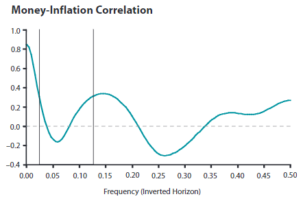
P.S. Here if we take logarithm to the equation of exchange, then we can get the relationship \( i_t \approx \pi_t + r_t \).
Also, if the output is relatively stable \( y_t=y\), then \( p_t=\frac{m_t}{y}\) (price level or is directly affected by money. Or if taking the logarithm, the inflation rate is one-to-one affected by the growth rate of money). P.S. the close to one relationship only works in the long run, see Wen (2006).
The empirical evidence of the relationship between excess reserves and the velocity of money can be found. In the figure, those two variables are negatively correlated.
Government Deficits Cause Inflation
Here, I would apply the equation of exchange and government budget constraint to explain how inflation is generated by government deficits. Recalling the government budget constraint,
\overbrace{p_t g_t}^{Gov Spending} + \overbrace{i_t d_t}^{Interest Payment} =
\underbrace{(d_{t+1}-d_t)}_{Increase in Debt Position}+\underbrace{T_t}_{Tax Revenue}+\underbrace{m_t-m_{t-1}}_{Print Money}
devide by \( p_t\) to get the equation in the real term,
$$ g_t+i_t \frac{d_t}{p_t}=\frac{d_{t+1}-d_t}{p_t}+\tau_t+\frac{m_t-m_{t-1}}{p_t} $$
, where \( \tau_t=\frac{T_t}{p_t}\).
By denoting real government debt as \( \hat{d}_t=\frac{d_t}{p_{t-1}}\), and replace \( (1+r_t)=(1+i_t)\frac{P_{t-1}}{P_t}=\frac{1+i_t}{1+\pi_t} \) and \( m_t = p_t y_t \), then we get all variables are in real terms,
$$ g_t – \tau_t +(1+r_t)\hat{d}_t =\hat{d}_{t+1}+\frac{p_t y_t-p_{t-1}y_{t-1}}{p_t}$$
At the steady state \( g_t=g_{t+1}=g, \tau_t=\tau_{t+1}=\tau \) and so on, and thus,
$$ \underbrace{g+r\hat{d}-\tau }_{Growth\ of \ interest\ deficits}= \underbrace{\frac{p_t-p_{t-1}}{p_t}}_{Seignorage} \times y$$
From the above equation, we can find that if inflation increases then it means the RHS increases. The LHS consists of two parts. Government Spendings \( g + r\hat{d}\) and government revenues \( \tau \). That means the government is getting deficits if the LHS rises. Meanwhile, the RHS increases and so inflation grows.
In sum, we find that government deficits, in the long run, would induce inflation. The zero-inflation condition is to make the LHS of the equation equal to zero (government spendings offset government revenue).
Reference
Wen, Y., 2006. The quantity theory of money. Monetary Trends, (Nov).