Learning – Page 10

The Neutrality of Money

Assume the cash-in-advance constraint always binds $(x_{t+1}=0)$.

Still, private sectors maximise their utility s.t. budget constraint and cash-in-advance constraint. Let’s also include labor as a disutility and assume output is produced by labour.

$$ \max_{c_t, b_{t+1}, x_{t+1}} \sum_{t=0}^{\infty}\ \beta^{t} [u(c_t)-v(l_t)] $$

$$ p_{t-1}y_{t-1}+b_t(1+i_t)+x_{t}-T_t=x_{t+1}+p_t c_t+b_{t+1} $$

$0 \leq x_{t+1}$

$$ 0 \leq l_t \leq 1 $$

, with $ y_{t-1}=l_{t-1}$

Now the output is not exogenous anymore but depends on an agent’s willingness to work.

F.O.C.

w.r.t. $c_t: \quad u'(c_t)=\beta (1+i_{t+1})\frac{p_t}{p_{t+1}}u'(c_{t+1}) $

w.r.t. $l_t: \quad v'(l_t)=\beta u'(c_{t+1})\frac{p_t}{p_{t+1}} $

At the steady state, $ \frac{p_t}{p_{t+1}}=\frac{1}{1+\pi}$ and $y_t=l_t=c_t=y$ (output is equal to labour’s production in the long run). The output could be calculated as the following equation. (at the steady state means in the long run).

$v'(y)=\beta u'(y)\frac{1}{\pi}$

Therefore, we can find that,

Money is netural: if change $ m $ (stock of money, or money supply), then output is not affected. For example, if money doubles in all time, the fraction $ \frac{p_t}{p_{t+1}}$ keeps constant. No affecting the real term of output $ y$.
Moeny is not super netural: if change $\pi$ (inflation rate), then output would change. (y decrases if $\pi$ increases. That can be analysed by the curvture of $ v$ and $ u$ functions).

Question: First we assume cash-in-advance constraint binds. The QTM states that $ growth rate of money$ and $inflation $ is one-to-one correlated only if assuming /(y/) is stable ($m_t=p_t y$). However, we find the relationship between inflation and output here. There seems a contradiction of whether fixes $y$ or not. So, how to bridge the connection between inflation and money growth?

Answer: From the demand point of view or the Cash-in-Advance constraint ( $p_t c_t=M_t, or x_t=0$ by our previous assumption ). At the steady state, consumption is stationary, so $ \frac{M_t}{p_t}=\frac{M_{t+1}}{p_{t+1}}= \frac{M_{t+2}}{p_{t+2}} =…$ imply the stock of money and price level are connected, and so the connection between growth rate of money and inlfation works. The inspiration is the cash-in-advance constraint binds, and we consider the problem by fixing consumption in the long-run stationary condition.

The question and answer also state that the neutrality of money bases the key cash-in-advance assumption.

Empirical study examples are as McCandless and Weber (1995)

Reference

McCandless, G.T. and Weber, W.E., 1995. Some monetary facts. Federal Reserve Bank of Minneapolis Quarterly Review, 19(3), pp.2-11.

A Cash-in-Advance Model

Here, I would use the cash in advance model to illustrate some economic phenomena.

Assumptions

Two core assumptions of the cash in advance model. 1. People need cash to purchase goods. 2. Income is received with a lag. The main implication of those two assumptions is that people cannot use the proceeds from the current sales to fund the purchases because people cannot get income back immediately but in the next period (e.g. employees earn wages with a lag).

Market Players

Before talking about the model, I would first illustrate the balance sheet of three main players in the market, the central bank, the government, and the private sector.

Monetary Authority or the central bank faces a simplified budget constraint,

$$ \hat{b}_t (1+i_t)+m_t=\hat{b}_{t+1}+m_{t-1}+tr_t, \quad t=0,1,2,… $$

$ \hat{b}_t $ denotes the hodling of government bonds
$ i_t $ is the nominal interest rate
$m_t$ is the money stock
$tr_t$ are transfers to the government

Fiscal Authoristy or government face the following constraint,

$$ T_t+tr_t+\hat{d}_{t+1}=\hat{d}_t (1+i_t)+p_t g_t $$

$ \hat{d}_t$ denotes the government debt
$ T_t$ are tax revenues
$ g_t$ is (real) government purchases
$ p_t$ is the price level

LHS represents the assets, and RHS represents the liability.

If consolidate those two constraints together, then we get the public sector Budget Constraint,

$$ T_t+(\hat{b}_t-\hat{d}_t)(1+i_t)-m_{t-1}=(\hat{b}_{t+1}-\hat{d}_{t+1}-m_t+p_t g_t) $$

If define $ D_t=\hat{d}_t+m_{t-1}-\hat{b}_t $ as the net position of public sector debt, then we get,

$$ \underbrace{T_t}_{taxes}+ \underbrace{(D_{t+1}-D_t)}_{deficit}+\underbrace{m_{t-1}i_t}_{seignorage}=\underbrace{i_t D_t}_{interest}+\underbrace{p_t g_t}_{spending} $$

Or if define $d_t=\hat{d}_t-\hat{b}_t$ (, which can be considered as the net position of government debt, the net amount runing in private sectors), then

$\underbrace{T_t}_{taxes}+ \underbrace{(d_{t+1}-d_t)}_{deficit}+\underbrace{(m_t-m_{t-1})}_{seignorage}=\underbrace{i_t d_t}_{interest}+\underbrace{p_t g_t}_{spending}$

P.S. Serignorage behaves like the tax of inflation? See the reading in the end.

Private Sectors: Consider that private sectors have an endowment $y_t$ each period, and they would sell the endowment to get cash, $p_t \cdot y_t$, in the subsequent period. Private sectors then have to use those cash to buy endowments (goods and services). The private sectors face a budget constraint as the following,

$$ p_{t-1}y_{t-1}+b_t(1+i_t)+(M_{t-1}-p_{t-1}c_{t-1})-T_t=M_t+b_{t+1} $$

$$ p_t c_t \leq M_t $$

, where $ b_t $ is the government bond and $ M_t $ is the money holding.

If define $ x_{t+1} = M_t – p_t c_t $, which means the excess cash holding, then the budget constraints of private sectors are,

$$ p_{t-1}y_{t-1}+b_t(1+i_t)+x_{t}-T_t=x_{t+1}+p_t c_t+b_{t+1} $$

$x_{t+1} \geq 0$

LHS are the source of money at period $t$, and RHS are how the private sector uses those money. The private sector can use the money to (1) consumer, (2) buy bond and earn interest, and (3) simply hold the money

Private sectors maximise their lifetime utility subject to budget constraints.

$$ \max_{c_t, b_{t+1}, x_{t+1}} \sum_{t=0}^{\infty}\ \beta^{t}\cdot u(c_t) $$

$$ s.t. Two\ Constaints $$

Solve the problem by Lagrangian.

$$ \mathcal{L}= \sum_{t=0}^{\infty} \beta^t \{ u(c_t) \\ – \lambda_t ( x_{t+1}+p_t c_t+b_{t+1}-p_{t-1}y_{t-1}+b_t(1+i_t)+x_{t}-T_t ) \\ -\mu_t x_{t+1} \} $$

Take f.o.c.

$ \frac{\partial \mathcal{L}}{c_t}: \quad u'(c_t)=\lambda_t p_t $

$ \frac{\partial \mathcal{L}}{b_{t+1}}: \quad \lambda_t=\beta(1+i_{t+1})\lambda_{t+1} $

$ \frac{\partial \mathcal{L}}{x_{t+1}}: \quad \lambda_t -\mu_t=\beta \lambda_{t+1} $

Here, let’s focus on the second and the third equation. If $ i_{t+1} =0$, then $\mu$ has to be zero as well to make them equal. Also, by completementary slackness, if $ \mu =0$, then $x_{t+1}$ must be greater than zero.

The implication is that private sectors would hold excess cash (hoard cash) even if the interest rate is zero. That is the liquidity trap. Although the government adjusts the interest rate to be zero in order to stimulate the economy, people do not spend that money. Instead, people just hoard the money.

Euler Condition of Private Sectors

Combining three f.o.c., we can get the following Euler condition.

$$ u'(c_t)=\beta(1+i_{t+1})\frac{p_t}{p_{t+1}}u'(c_{t+1}) $$

$u'(y_t)=\beta(1+i_{t+1})\frac{p_t}{p_{t+1}}u'(y_{t+1})$

If markets clear, then $y_t=c_t$.

Competitve Equilibrium

The competitive equilibrium of this problem is a sequence of price $ \{ p_t,i_{t+1} \}^{\infty}_{t=0}$ and allocations $ \{ c_t, b_{t+1}, x_{t+1}, g_t, T_t, d_{t+1}, m_t \} $ such that given price,

The sequence $ \{ p_t,i_{t+1} \}^{\infty}_{t=0}$ solves the household’s problem.
Bond markets clear, $ b_t =d_t $.
Goods markets clear, $ y_t = c_t+g_t $.

Equation of Exhange

We here combine the private sectors and public sectors’ budget constraints and apply the markets clear condition, and then we can get,

$$ p_{t-1}y_{t-1}+x_t+(m_t-m_{t-1})=p_t y_t +x_{t+1} $$

Assume at the beginning period when $ t=0$, $ y_{t-1}=x_0=m_{-1}=0$. Thus,

$$ m_0=p_0 y_0 +x_1 $$

Similarly, in the following period,

$$ m_t = p_t y_t +x_{t+1} $$

The above equation is the equation of exchange, the one I mentioned in the blog: Quantity Theory of Money (QTM). It is called the Fischer equation or quantity equation.

Define $ v_t =\frac{m_t-x_{t+1}}{m_t} $, then we can get the QTM equation.

$$ m_t v_t = p_t y_t $$

Recall the liquidity trap. If in the liquidity trap, then $ i_{t+1}=0 $ and $x_{t+1}>0$ people hoard excess money. Therefore, the velocity of money $v_t <1$ .

However, if not in the liquidity trap, then $ i_{t+1}>0$, and $x_{t+1}=0 $ and $v_t=1$, so

$$ m_t=p_t y_t\ and\ p_t=\frac{m_t}{y_t} $$

P.S. Here if we take logarithm to the equation of exchange, then we can get the relationship $ i_t \approx \pi_t + r_t $.

Also, if the output is relatively stable $ y_t=y$, then $ p_t=\frac{m_t}{y}$ (price level or is directly affected by money. Or if taking the logarithm, the inflation rate is one-to-one affected by the growth rate of money). P.S. the close to one relationship only works in the long run, see Wen (2006).

The empirical evidence of the relationship between excess reserves and the velocity of money can be found. In the figure, those two variables are negatively correlated.

Government Deficits Cause Inflation

Here, I would apply the equation of exchange and government budget constraint to explain how inflation is generated by government deficits. Recalling the government budget constraint,

$\overbrace{p_t g_t}^{Gov Spending} + \overbrace{i_t d_t}^{Interest Payment} = \underbrace{(d_{t+1}-d_t)}_{Increase in Debt Position}+\underbrace{T_t}_{Tax Revenue}+\underbrace{m_t-m_{t-1}}_{Print Money}$

devide by $ p_t$ to get the equation in the real term,

$$ g_t+i_t \frac{d_t}{p_t}=\frac{d_{t+1}-d_t}{p_t}+\tau_t+\frac{m_t-m_{t-1}}{p_t} $$

, where $ \tau_t=\frac{T_t}{p_t}$.

By denoting real government debt as $ \hat{d}_t=\frac{d_t}{p_{t-1}}$, and replace $ (1+r_t)=(1+i_t)\frac{P_{t-1}}{P_t}=\frac{1+i_t}{1+\pi_t} $ and $ m_t = p_t y_t $, then we get all variables are in real terms,

$$ g_t – \tau_t +(1+r_t)\hat{d}_t =\hat{d}_{t+1}+\frac{p_t y_t-p_{t-1}y_{t-1}}{p_t}$$

At the steady state $ g_t=g_{t+1}=g, \tau_t=\tau_{t+1}=\tau $ and so on, and thus,

$$ \underbrace{g+r\hat{d}-\tau }_{Growth\ of \ interest\ deficits}= \underbrace{\frac{p_t-p_{t-1}}{p_t}}_{Seignorage} \times y$$

From the above equation, we can find that if inflation increases then it means the RHS increases. The LHS consists of two parts. Government Spendings $ g + r\hat{d}$ and government revenues $ \tau $. That means the government is getting deficits if the LHS rises. Meanwhile, the RHS increases and so inflation grows.

In sum, we find that government deficits, in the long run, would induce inflation. The zero-inflation condition is to make the LHS of the equation equal to zero (government spendings offset government revenue).

Reference

Wen, Y., 2006. The quantity theory of money. Monetary Trends, (Nov).

Notes on Seigniorage and Budget Constraints Download

The Fed’s Balance Sheet

Here we would try to understand the different components of the Fed’s balance, for the further study of policy impacts on the economy and the cash in advance model.

The fed’s balance sheet (H.4.1 report) is weekly updated every Thursday, and it presents the assets and liabilities of Federal Reserve Banks.

Assets

Fed’s assets are how the Fed uses money. Most of the money is spent on securities, unamortized premiums and discounts, repurchase agreements, and loans. For example, if the fed buys assets (MBS) or bonds (T-securities) by printing money, then those purchased investments are the assets of the Fed. The followings are some typical assets of the Fed that occupy a significant proportion.

Treasury Securities: Treasury Securities account for the highest proportion of the fed’s assets. They are consisted of the T-bills, T-notes, and T-bonds by maturity. Treasutry secuirities account for 64% of total assets, (5,533,219 million dollors).
Mortgage-backed Securities: MBS are securitisations of a basket of home loans. They occupy about 29% of total assets (2,527,824 million dollars).
Loans: Those are money borrowed by other commerical banks through repo or discount window. The discount window is simplised as that Fed lends money to those borrowers and chages for an interest rate, federal discount rate. Loans have 48,317 million dollars balance.

(Total assets are 8,574,871 million dollars.)

Liabilities

The liabilities of the fed represents how the money comes from, consisting of Federal Reserve Notes, Reverse repurchase agreements, and deposits.

Federal Reserve Notes: Paper currency (Federal Reserve notes) outstanding net of the quantities held by Reserve Banks. In short, they are net of money oustanding. The balance of it is 2,158,089 million dollars, which is about 25% of total liabilities of the Fed. From historial data, we can find that the money growth at relatively constant rate except during Aprial, 2020. The growth rate jumps.
Reverse repurchase agreements: Fed sells securities to a counterparty subject to an agreement to purchase back the securities at a later date. The Fed uses Repo or Reserve Repo to conduct open market operations. By Repo, the Fed can release liquidity into the financial amrket. In contrary, the Fed tightens liquidity by revsere repo.
The deposits, which is also call reserves, are amount of money deposided by commercial banks. The reserve ratio is proportion required in order to keep financial banks operating less risky, and it is also an important tool of the monetary policy. When reserve ratio decrese, then the money supply woul increase. The Board was reduced to zero on 26 March 2020.

Fed’s Tools

Securities held outright: Treasury security and MBS together consist of the Securities held outright. The increase in those is due to the QE by Federal Reserve. Since the financial crisis of 2008, the Fed started to use QE to boost the economy, through which it purchased a huge number of financial assets (especially long-term assets). That account increased dramatically as well during the pandemic.
Repos and Reverse Repos: Those transactions are between cash and Treasury securities (mostly short term ones). These open market operations support effective monetary policy implementation and smooth market functioning by helping maintain the federal funds rate within target ranges. Repo: the desk purchases securities from the counterparty subject to an agreement to resell the securities at a later date. Each repo is similar to a loan collateralised by securities, and temporarily increase the supply of reserve banlances in the banking system. Reverse repo is the opposite. The desk sells securities and reduce supply of money.
Reserve rate as I have discussed before.

Federal Fund Rate

The following content is directly copied from the FRED. Links would be attached in the reference.

The federal funds rate is the interest rate at which depository institutions trade federal funds (balances held at Federal Reserve Banks) with each other overnight. When a depository institution has surplus balances in its reserve account, it lends to other banks in need of larger balances. In simpler terms, a bank with excess cash, which is often referred to as liquidity, will lend to another bank that needs to quickly raise liquidity. The rate that the borrowing institution pays to the lending institution is determined between the two banks; the weighted average rate for all of these types of negotiations is called the effective federal funds rate. The effective federal funds rate is essentially determined by the market but is influenced by the Federal Reserve through open market operations to reach the federal funds rate target.

The Federal Open Market Committee (FOMC) meets eight times a year to determine the federal funds target rate. As previously stated, this rate influences the effective federal funds rate through open market operations or by buying and selling of government bonds (government debt). More specifically, the Federal Reserve decreases liquidity by selling government bonds, thereby raising the federal funds rate because banks have less liquidity to trade with other banks. Similarly, the Federal Reserve can increase liquidity by buying government bonds, decreasing the federal funds rate because banks have excess liquidity for trade. Whether the Federal Reserve wants to buy or sell bonds depends on the state of the economy. If the FOMC believes the economy is growing too fast and inflation pressures are inconsistent with the dual mandate of the Federal Reserve, the Committee may set a higher federal funds rate target to temper economic activity. In the opposing scenario, the FOMC may set a lower federal funds rate target to spur greater economic activity. Therefore, the FOMC must observe the current state of the economy to determine the best course of monetary policy that will maximize economic growth while adhering to the dual mandate set forth by Congress. In making its monetary policy decisions, the FOMC considers a wealth of economic data, such as: trends in prices and wages, employment, consumer spending and income, business investments, and foreign exchange markets.

The federal funds rate is the central interest rate in the U.S. financial market. It influences other interest rates such as the prime rate, which is the rate banks charge their customers with higher credit ratings. Additionally, the federal funds rate indirectly influences longer-term interest rates such as mortgages, loans, and savings, all of which are very important to consumer wealth and confidence.

Key Takeaway: The Fed can adjust the effective federal fund rate by Open Market Operation, QE, etc.

Reference

Fed’s statement until 10 Nov 202`1: https://fred.stlouisfed.org/release/tables?rid=20&eid=1194154#snid=1194156

A good explanation of Repo: https://www.bankrate.com/banking/federal-reserve/why-the-fed-pumps-billions-into-repo-market/

https://fred.stlouisfed.org/series/DFF#0

https://www.newyorkfed.org/markets/domestic-market-operations/monetary-policy-implementation/repo-reverse-repo-agreements

Quantity Theory of Money (QTM)

My current reviews of how the aggregate demand curve is determined and how is the development of Keynesianism and Monetarism encourage me to get further insights into QTM, which is also one of the oldest and currently surviving economic theory.

Karl Marx

Let’s begin the story with Karl Marx who is not the pioneer of QTM but partially believed it. His idea about money is that the amount of money in circulation is determined by the quantity of goods times the prices of goods.

Keynes

John Maynard Keynes also agreed on part of the QTM, but he held a different opinion about the determinant of the quantity of money. He thought that the amount of money depends on the purchasing power or aggregate demand.

Keynes also thought output and velocity (k) is not stable in the short run. (coincide with his idea of price is super sticky in the very short run)

The Cambridge equation formed as the following,

$ M^d=k \cdot P \cdot Y $

Alfred Marshall, A.C. Pigou, and John Maynard Keynes assumed that money demand is determined by $k$, which represents a percentage of money hoarded in hands, times the nominal income $ P\cdot Y$.

P.S. Dr. Rendahl at Cambridge taught that part in S201 Applied Macroeconomics before, but I did not get it when I am as a student. Liquidity traps would be introduced in a later blog.

Friedman

Friedman held the similar idea with Keynes that the velocity would not fixed in the short run. He also stated that the velocity might not offset the effect of money growth, instead velocity moves in the same direction and reinforece with money growth empircally. For example, when quantity of money increase, the velocity rises as well (p.s. my idea: is that still true during the covid crisis? The U.S. example might not be the case, but needs data to prove).

In summary, Marx, Keynes, and Friedman all agreed with the quantity theory of money, but they have different ideas. Marx emphasised the productions, Keynes the demand and income, and Friedman the supply or quantity of money.

Empircal Study

Here are a maths and empircal studies.

$ M\cdot V=P\cdot Y $

In the long run, velocity and real output are constant, so money supply is positively correlated with the price level. However, in the short run, the output is not fixed, so changes in the money supply would change the real output.

By log transformation,

$ m+v=p+y $

$ v=p+y-m $

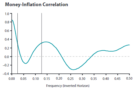
So the changes in velocity are determined by three parts, inflation, real output growth, and money growth. As shown in the figure below, some emprical data tell that correlation between money growth and inflation (y-axis) is close to one, about 0.82 exactly (as frequency is close to 0, means infinite long time period). Where the frequency (x-axis) means the frequency of periods used into the study. 0.5 frequency means horizon of changes in 2 periods (one period is a quarter as data are quarterly recorded). This study tells that in the long run, inflation is correlated with money growth, but the correlation is not that clear in the short run.

Ideas

By the Cambridge method, quantity of money is determined by people’s income times a portion $k$, and that $k$ would definitely changable with the macroeconomic condition. For example, in the recession, people are more likely to hoard more money for security reason, even interest rate is close to zero by liquidity trap. How that $k$ is determined, orhow to meature it? Also, how government and central banks’ policy could change people’s willingness of holding money?

Reference

Marx, K., 1911. A contribution to the critique of political economy. CH Kerr.

Wen, Y., 2002. The business cycle effects of Christmas. Journal of Monetary Economics, 49(6), pp.1289-1314.

Wen, Y., 2006. The quantity theory of money. Monetary Trends, (Nov).

Keynesianism, Monetarism, and Austrian School

Two extremes of economists, one group includes Keynesian economists who think the economy should be managed by intervention, and the other includes such as monetarists who believe the economy could self-adjust to equilibrium itself and do not need interventions.

Keynesian

The interventionists include Karl Marx and John Maynard Keynes. In 1936, Keynes published a book The General Theory of Employment, Interest, and Money. He challenged the classical economists that insisted that the economy would self-correct over time. Instead, Keynes considered that government should intervene in the economy by government spending in the short run. Instead of waiting until the economy is back on the right track, the government should actively stimulate by such as government spending (multiplier effects would result in more output. Marginal Propensity to Consume MPC less than 1 could result in the multiplier effects in IS model).

For example, if consumers spend less (consumption decreases), then the government could increase government spending and increase the money supply to boost the economy in recession. Consider

Critics: Some opposite ideas are there. Government spending may not efficiently increase the economy. For example, as in the Broken Window Fallacy, if a window is broken, then a series of jobs and works are created. The householder spends money to pay the worker who fixes the window. The worker then gets money to spend it…etc. However, those created jobs and works are actually wastes, because the window does not have to be broken to make the series of works happen. The householder can spend money on other things he wants.

Are Government spendings similar to the broken window? Maybe it is not. If government spend for indeed useful things such as public university, national defense, then government spendings do create jobs. However, if gov spends on useless things such as deliberately breaking a window and fixing it, then the economy would be inefficient, through current jobs are created. In the meantime, if the government spends on useful things in the beginning but the sub-things are useless in the following chain, then Broke Window Fallacy comes again.

In addition, if the government needs to borrow money to finance the spending, then crowding out effects also exist that private investment and consumption are crowded out or reduced. Because government borrowings bring fewer loanable funds and higher interest rates. The higher the interest rate, the higher the cost of investment.

In summary, Keynesian thinks the government should react to stimulate the economy in recession, decrease the unemployment rate and increase the growth of the economy by government spending (Expansionary Fiscal Policy). It is generally agreed that the Keynesian idea that an increase in government spending does help to make the economy leave recession in the short run. However, the trade-off is the long-run development, and it cannot be captured in current economic theory. Further studies are needed.

P.S. Gov always prefers Keynesianism in facing depression.

New Keynesian

Similar to the new classical, new Keynesian also assume households and firms maximise their own expected utility with rational expectation. The difference is that the new Keynesian assumes also a market failure because markets are not perfectly competitive in price and wage. Thus, prices and wages become “sticky” that fails to adjust with the economic conditions.

The sticky price is one of the reasons that the economy cannot achieve full employment. Therefore, fiscal policy and monetary policy could stabilise the macroeconomy and achieve an efficient macroeconomic outcome.

Coordination Failure is another important new Keynesian concept to explain the recession and unemployment. The invisible hand fails to coordinate the usual, optimal, flow of production and consumption. See further studies.

Labour market failure: Efficiency wages also explain the unemployment condition. That theory aims to explain the long-term effect of previous unemployment on permanent unemployment in the long run. (See E200 notes). Shapiro and Stiglitz (1984) developed the shirking model, and their works contribute to the explanation of the employment rate.

See notes of E200.

Taylor rule describes the relationship between the nominal interest rate (, which is set by CB), and other economic factors. Those factors are inflation, output, economic condition (Taylor, 1993).

$$ i_t=\pi_t+r_t^* + a_{\pi}(\pi_t -pi_t^*)+a_y (y_t-y_t^*) $$

In short, the nominal interest rate is affected by inflation, and how the economy deviates from the target.

Some central figures of the new Keynesian areGregory Mankiw, Stanley Fischer, and Jordi Gali.

Monetarism

Fewer interventionists are groups of economists who believe the government and central bank should not interact with the economy operating. Those economists include such as monetarism and the Austrian School of economics. Monetarism is the economic theory focusing on the money supply and central banking system.

Milton Friedman, a Nobel Prize holder and professor at the University of Chicago, is one of the most famous proponents of monetarism (classicalism). He holds different opinions from Keynes and those Cambridge economists who consider money demand determines the amount of money in the market. Instead, Friedman emphasizes the importance of the money supply from the central bank. (Look at the blog post about the Quantity Theory of Money, QTM.)

(M\cdot V=P\cdoc Y \)

In the long run, if the central bank creates too much money into the economy, then there are too much money and too little supply of goods. Price would increase and so inflation would increase. That would result in inefficient resource allocation because consumers do not know whether the increase in price is from inflation or from goods and services becoming more valuable. Monetarists do not agree to create too high inflation even though it can increase outputs in the short run, because consumers would recognise the increase in the price level in the long run, and then the price level goes high.

monetarists agree 2% to 3% level increase in money supply or inflation is healthy. As central banks always prefer Keynesianism to stimulate economic growth, monetarists use rules to constrain the power of the central bank.

Classical Theory

The classical theory is firstly formed by Adam Smith. The classical idea states that consumers and firms make decisions in the free market to maximise their own benefits, which are utility and profits. The invisible hands would fix the market itself without any interventions.

The base stone of classical theory is “flexible wages” that wages would increase with inflation and decrease with deflation. However, Keynesian economists believe the price is sticky in the short run.

Ideas:

Two (or several) countries’ comparisons to find the long-run effects of Keynesian policy. —- DiD or other causality testing method.
U.S. Gov reacts to the Covid-19 by fiscal policy (government spending and helicopter drop) and monetary policy (lower the federal fund rate) and those policies both boost aggregate demand. However, without any increase in factor inputs and significant technology progress, the aggregate supply is frustrated due to unemployment (probably due to increasing in resource price but I have not investigated). Policies did not really result in hyper-inflation largely because consumers are less confident and unwilling to spend money (MPC is too low), though there is a government spending increase and low-interest rate to boost investment. Economy is current not bad (or maybe its bad). However, it is terrible in the long run. Uncertainty about the future price level and may lose credibility of U.S. dollar. Idea: why no hypter inflation? (my idea is credibility and dollar-oil system).
China case is different. Sustainable supply (I might think it partially due to the system of organisation of country. Of course, there are complex reasons) and frustrated demand that people do not have enough willingness to spend money on normal goods (however some luxury goods have increasing demand even with price tag rising). Ideas: 1. China consumption structure. Different demand elasticity toward differnt goods. Also, elasticities vary over time. Considering an elasticity index? 2. Potential problem, the broken window fallacy.
People worried about the stagflation. Theoritically, it should happen in the U.S., but the stagflation seems is delaied or alliviated, probably because the effect is absorbed by other countries such as Canada —- Due to U.S. dollar’s credibility. For China, I personally might not think stagflation would happen in China. As supply is still not bad.

Austrian School of Economics

Carl Menger is considered to be the founder of the Austrian School. The Austrian school focuses mainly on people, their incentives and limited knowledge (including legal, social, cultural, political, and economic institutions). How individuals make decisions constitutes Austrian economic thought. Thus, they emphasise the ever-changing and adaptive nature of the economy.

F.A. Hayek was a leading member of the Austrian School of Economics, and he believed that the prosperity of society was driven by creativity, entrepreneurship, and innovation, which were only possible in a society with free markets. The Nobel prize was awarded to him and Gunnar Myrdal in 1974 for their pioneering work in the theory of money and economic fluctuations and for their penetrating analysis of the interdependence of economic, social and institutional phenomena.

Austrian school emphasises supply and productivity in the recession, while Keynesianism emphasise demand.

Joseph Schumpeter

Schumpeter became known for his original ideas regarding entrepreneurship and “Creative Destruction”.

The Library of Economics and Liberty immortalizes him thus: “Schumpeter pointed out that entrepreneurs innovate not just by figuring out how to use inventions, but also by introducing new means of production, new products, and new forms of organization. These innovations, he argued, take just as much skill and daring as does the process of invention.”

His work venerated entrepreneurship and innovation, arguing that entrepreneurs improve our lives by developing new, unheard-of industries or improving existing goods and services. This foundation is important to remember, as his work does postulate that capitalism is bound to decay into socialism over time.

Schumpeter’s The Theory of Economic Development describes an evenly rotating economy of a stationary state. Within this imaginary state, there is no room for innovations and innovative activities, because these activities would disturb it, causing it to no longer be a stationary state. Innovation is the solution to this state.

Policy Responses to COVID 19 by Country

https://www.imf.org/en/Topics/imf-and-covid19/Policy-Responses-to-COVID-19

Reference

https://youtu.be/xKGtmzLP8gw

https://youtu.be/cqzRAy-mJtU

Joseph Schumpeter: the most important economist you might not know of

Friedrich August Hayek

Market Efficiency And Anomaly

Background: Efficient Market Hypothesis

The efficient market hypothesis generally states that the asset price has already reflected all the information (Fama, 1998).

This implies the stock price depends on all fundamentals and includes all information existing in the market. Any small deviations might be quickly diminishing with new information coming out. Therefore, the EMH rules out the profitable investment opportunity in the market, because the price is already the right price.

Is the market efficient or not?

The price might be incorrect in the real market. Actually, the anomaly, which is the deviation of the strategic price from the expected true price, seemingly does exist. Then an issue arises:

Whether the investor could beat the market?

To address this issue, we apply an asset pricing model such as CAPM to calculate the expected benchmark return we should get subject to some factors.

The anomaly can be expressed as:

$\alpha=r_{real}-r_{benchmark}$

This equation shows that alpha (anomaly), which is the alpha in CAPM, is the real-world return less the benchmark return.

Then, the efficiency can be examined by testing the existence of an anomaly. If an anomaly exists, it means the market is not quite efficient. Therefore, investment strategies could be applied to earn the abnormal return and beat the market. This test can be conducted by constructing a regression model as, $r_{i,t} =\alpha+r_{f,t}+\beta \times (r_{m,t}-r_{f,t})$ and do joint hypothesis testing.

Here are some relative literature introducing that the market is inefficient. Schwert (2003) stated that the market is not efficient, indicated by the existence of anomaly; Jensen (1978) proofed the inefficiency after adjusting the inconsistent data and missed techniques; Latif et al. (2011) also demonstrated different types of anomalies generated from technical, fundamental and behavioural aspects.

Given that the market is inefficient, the question now is how investors could earn the abnormal profit.

How could investors earn the abnormal profit?

The strategy is to construct a financial portfolio earning the abnormal return (anomaly), and in that strategy, investors select stocks based on their certain characteristics. (two examples below).

The momentum strategy: stocks that performed well in the previous period would also outperform others in the following period (Jegadeesh & Titman, 1993). The contrarian effect is the opposite.

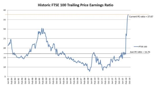
The value investing strategy: stocks with a high P/E ratio or P/B ratio are overvalued, vice versa. Stocks with such as low P/E ratio, Dividend Yield, P/B ratio, etc. are generally under-priced. Thus, buying those cheap stocks could result in a profitable opportunity.

There are numerous investment strategies as we discussed above, and investors could simply apply one strategy or even combine some of the strategies to construct a portfolio to beat the market.

How to test ‘beat the market’?

Applying back-testing to simulate the portfolio’s performance

back-testing is the methodology by which people can see the performance of a certain strategy by some historical data (Campbell, 2005). Here is an example of back-testing below:

Firstly, investors could sort stocks by strategy. If they apply the momentum strategy, they simply sort stocks’ historical return $ (r_{t=1,i}) $ from high to low. Then, investors would make the quartile cut-off, selecting stocks in the first quartile (best-perform stocks) and keeping them into the next period. This periodical return would be the strategic return. After that, we sort the second period return $ (r_{t=2,i}) $, select a first quartile stock again, and keep them into the next period again and again.

Under this procedure, we could use the historical data to track strategy periodical performance. Then, we could examine the existence of an anomaly by subtracting strategic return from the benchmark return.

Reference

Campbell, S.D., 2005. A review of backtesting and backtesting procedures.

Fama, E.F., 1998. Market efficiency, long-term returns, and behavioral finance. Journal of financial economics, 49(3), pp.283-306.

Fama, E.F., 1998. Market efficiency, long-term returns, and behavioral finance. Journal of financial eco

Jegadeesh, N. and Titman, S., 1993. Returns to buying winners and selling losers: Implications for stock market efficiency. The Journal of finance, 48(1), pp.65-91.

Jensen, M.C., 1978. Some anomalous evidence regarding market efficiency. Journal of financial economics, 6(2/3), pp.95-101.

Latif, M., Arshad, S., Fatima, M. and Farooq, S., 2011. Market efficiency, market anomalies, causes, evidences, and some behavioral aspects of market anomalies. Research Journal of Finance and Accounting, 2(9), pp.1-13.

Lux, T. and Marchesi, M., 2000. Volatility clustering in financial markets: a microsimulation of interacting agents. International journal of theoretical and applied finance, 3(04), pp.675-702.

Schwert, G.W., 2003. Anomalies and market efficiency. Handbook of the Economics of Finance, 1, pp.939-974.

Hello world!

Welcome to WordPress. This is your first post. Edit or delete it, then start writing!