Taylor Rule

Developed by John B. Taylor – aims to be a rule of thumb

If the Federal Reserve decides to increase the liquidity, it would then buy bonds and put more money into the market. As there is more money to lend, the interest rate would go down.

The monetary policy aims to target the inflation rate. Considering the Philips curve, there is a trade-off between unemployment and inflation. Unemployment could be replaced by its counterpart, economic growth. We consider the goal of the monetary department to balance GDP and Inflation.

The Fed normally has a target interest rate, the federal funds rate, which is the overnight rate in the interbank market for short term lending. How should the monetary policy set the target interest rate? This is the key discussion of the Taylor rule.

$$i=i^*+a (\pi – \pi^*) – b(U-U^*)$$

By the Philips curve, we replace unemployment with output. As we separate the interest rate to be the real interest rate and the inflation rate.

$$ i=r+\pi^*+a\underbrace{(\pi-\pi^*)}_{Inflation\ Gap}+b\underbrace{(Y-Y^*)}_{Output\ Gap} $$

The output gap could be considered to be by what percentage of the current GDP is below the Potential GDP.

Clearly, the Taylor rule is intuitively to be correct.

If there is an inflation gap the current inflation is greater than the target, which also means there is an extra money supply moving the CPI upward, then the Fed should conduct a contractionary monetary policy, and it should set a higher interest rate.

If the GDP growth is lower than the target (potential), or if the unemployment rate is greater than the target, then the Fed would like to stimulate the market. Thus, it would decrease the interest rate.

For the Taylor rule, John Taylor did not mean the monetary policy should follow it. It is not a law but just a rule of thumb. Normally, we also set the coefficients \(a\) and \(b\) to be 1\2. However, if we think the government would pay more attention to the inflation target, then we could certainly increase the weight of inflation gap.

Bernoulli’s Inequality

$$lim_{x\rightarrow 0}(1+x)^n ~ 1+nx$$

Proof:

Taylor Expansion at x=0

$$ (1+x)^n\approx (1+x)^n|_{x=0} + \frac{d (1+x)^n}{d x}|_{x=0} \times (x-0) + \frac{d^2 (1+x)^n}{d x^2}|_{x=0}\times (x-0)^2 + O(x^3) $$

$$ \approx 1 + nx + \frac{n(n-1)}{2} x^2 + O(x^3)$$

$$ \approx 1 + nx + O(x^2)$$

George Soros & the Japan Market

The story began in the third quarter of 2012 when the Japanese Yen depreciated until the beginning of 2013 as the rising Blue curve shows.

As we all know, Japan has been getting into a negative interest era for a long time, partially because the terrible economic condition makes its government have to raise debts (I haven’t studied the Japanese problem. Once do that, I will update it.).

Since 2008 when the US saved the market through QE, the Japanese CB chose to conduct a similar monetary policy to boost its domestic market after Aben won the presidency.

Intuitively, Abenconomics applied QE would result in an excess supply of the Japanese Yen. Unlike the US dollar that backed with the Oil price, the excess money supply of the Japanese Yen would make it depreciate. Soros estimated that opportunity and shorted the Yen, and meanwhile took a long position of Nikkei stocks and bonds in the Japan Market.

QE would result in an extra money supply as we all know, investors who get that extra money would try to invest that money into the financial market, both the stock market and the debt market. As we can find that stock market increased with the depreciation of the Japanese Yen. Soros won the gamble.

However, there is a Winner and there must be a loser, which is the Japanese Central Bank. The failure of the monetary policy of the Japanese CB made worse its domestic economic condition.

In the current world, the CB of each country has to rigorously implement its monetary policy. QE might not be an ideal way to stimulate the market, because not every currency has the ability, like the US dollar, to back up with commodities and oil prices. Also, countries especially those that are in the EU are facing a conflict of interest in conducting monetary policy.

US Dollar & Commodity Price

The line chart below shows the relationship between US Dollar Index and Commodity Price Index.

The dynamic macroeconomic condition of the world drives me to find the correlations among some macroeconomic indices.

Rising Energy Price and Commodity Price

The tight relationship between Russia and Ukraine (and NATO) and the pandemic drive energy price such as crude oil and gas keep increasing. On one hand, I may consider the rising energy price as mainly a supply-side problem. Although European countries conduct sanctions on Russia, they still have relative rigid demand for gas and crude oil from Russia. The lack of energy from the EU pushes the oil price to rise as the Green Line shows in the Figure below. On the other hand, the tight Global relationships between huge parties such as Russia, US, the EU, and China enhance the needs of necessities. Therefore, the prices of commodities and oil, which are necessities not only for the downstream consumers but also for industries, increase as expected.

Those facts that positive correlation of commodity price, energy price, and crude oil price can be found in the Figure below.

US Dollar Index and Commodity Price

Intuitively,

As the US dollar is internationally admitted and exchanged currency, commodities and crude oils are priced by it (the US Dollar).

As shown in the Figure below, there seems a negative correlation between the US dollar index and the Commodity index.

One explanation of that negative relationship is that the value or the intrinsic value of a commodity is the same either priced by the US dollar or price by the British pound. Therefore, if the US dollar depreciates, then people should spend more US dollars to buy the same certain quantity of commodities. Similar logic could be found in crude oil prices.

There could be other explanations or other factors that could be taken into consideration. Under the current world condition that de-globalisation and uncertainty emerge, people would hold more safe assets. Thus, commodities and old, which are necessities, and gold, which is a generally accepted symbol of value, become the top safety consideration for people (investors and firms may have greater demand for commodities and energy, and normal people may get access to gold and have more demand for gold). Finally, the price of them increases.

However, there raises a question I haven’t yet spent time on studying it.

If the US dollar appreciates, then the price of commodity should decrease as I just introduced. Then, there might be more demand for commodities and oil as the price is getting low (you may say the low price is due to the appreciation of the US dollar. you are right maybe, but that cannot convince me), at least in the U.S. market. As the transaction is made with the US dollar, the more demand for commodities and oils means more demand for the US dollar, therefore US dollar should keep appreicating. Is that right? If it is, then there won’t be a convergence and won’t have an equilibrium, instead, the appreciation of the US dollar would be magnified. The reverse situation would happen if the US dollar depreciates.

Emerpically,

The Fred commission announced to increase the interest rate, in order to face the hyper-inflation resulting from its previous quantitative easing. Increasing interest rate means the US market would be more attractive to Global investors, so an increase in demand for the US dollar drives the US dollar to appreciate. The commodity price logically should go down. However, that divergence does not come out as we can find in the figure since the tight relationship between Russia and Ukraine happened.

Why the empirical finding contradicts with our logical indication?

Is that a result of the safety consideration (that people worry about the war and start to hold necessities) we just mentioned? If it is, then how can we split that part of the effect and show the negative correlation between the US dollar and commodity price. If not, then what factors contribute to the conflict? Is that due to the reason I discussed above? or there are any other factors (of course there are, but I neglect them because they have relatively small effects) cause that phenomenon?

Crisis

In the second figure, the crisis happened in 2008 and 2019-now, as shown in the shaded period. In the crisis, the commodity price seems a leading index of the US dollar. The commodity reflects prior to the other economic factors, as demanders of the commodity, production firms, need to avoid fluctuations of prices. So they make hedging transactions earlier and predict the commodity price so that they can apply to their production process smoothly.

荷兰农业 v.s. 中国农业

1. 背景

荷兰农业出口额仅次于美国,位列世界第二。但荷兰国土面积仅占美国1/270。

2. 基本条件

  • 天然气 荷兰纬度与我国黑龙江接近,地理环境导致荷兰气温低,对于农业为劣势。
  • 育种业 保障全年生产新品种
  • 机器自动化 通过计算机自动控制温度 湿度等,研究 不同光线对作物生产的影响等 以提高单产。

  • 农业人口少 1% 与美国农业人口类似。
  • 荷兰出口额ranking:1. 花卉 2. 肉 3. 蛋、奶 4. 蔬菜 5. 水果 6. 酒 7. 谷物等副产品 etc
  • 蔬菜仅占rank3

3. Finding

研究 – 提高产值的方法

规模效应 – 人少 -人均高

4. 中国农业 v.s. 荷兰农业

观点来自参考资源,未研究数据严谨性,仅作为思考inspiration

荷兰农业为赚钱 v.s. 中国农业为了维持社会稳定

我国农业为了维护公平 保证employment。于是限制资本进入农村,以保护农民利益。

即使科技技术引进可以提高产能,但是为了避免利润被大农业公司榨干,因而给予限制。

商业机构在整条产业链上寻求利润,因为最上游生产端被限制进入,于是从下游终端介入,通过互联网平台与菜贩子竞争利润空间。

公平 – 保证employment <- 我国为保 就业+稳定 而限制商业进驻农业生产上游

效率 – 科技 + 管理带来规模效应 <- 被选择性舍弃

5. Inspiration

在 公平 和 效率 之间取舍。 放弃了效率,放弃了市场的选择,为了保证贫富差距,为了保证就业公平

本源 1. 人口: 人口多 人均少。2. 教育:部分群体受教育程度不足以在城镇化转型中获得工作机会(prob农业) <-> 教育同时意味着 人才相对缺失。 3. 市场:由于上游限制,人才不愿意进入农业生产,因为没有profitable opportunities。人才并非为regulation的原因而缺少。4. 城镇 制造业+服务业 无法吸收农业人口的转移

基于 1. 人口。 城镇的制造业+服务业 无法吸纳农业人口转移,也因此 为保证 公平 农业人口数量不能减少 以将土地租给高效的生产管理人员。

6. Reference

https://www.bilibili.com/video/BV1Fr4y1a7ua?share_source=copy_web

货币+信用 分析

一般来讲(参考“宽信用阶段哪些行业会有超额收益?”)宽货币+宽信用 or 紧货币+紧信用为目标状态。即 货币为政策的工具(为实现货币政策目标),信用为市场方向。当政策与市场同向,可以理解为政策工具即货币的调整使得市场达到想要的效果。

那么 宽货币+紧信用 and 紧货币+宽信用 即为达成货币政策目标的中间态。

我国经济情况总体为控制风险,宽货币大多仅在为刺激经济发展时出现。当前国内经济不景气,中央政策刺激经济发展而采取增加专项债、针对小微企业贷款释放等政策。但是银行为了限定违约率往往难以执行这些政策。

但是具体行业对宽货币宽信用的反应难以一概而论。

宽货币:降准 降息 etc

Isoquant

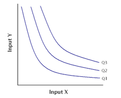
An isoquant map where production output Q3 > Q2 > Q1. Typically inputs X and Y would refer to labour and capital respectively. More of input X, input Y, or both are required to move from isoquant Q1 to Q2, or from Q2 to Q3.

MRTS equals the slope of the Isoquant.

Difference with the Indifference Curve

Isoquant and indifference curves behave similarly, as they are all kinds of contour curves. The difference is that the Isoquant maps the output, but the indifference curve maps the utility.

In addition, the indifference curve describes only the preference of individuals but does not capture the exact value of utility. The preference is the relative desire for certain goods or services to others. However, the Isoquant can capture the exact number of production.

Shape of the Isoquant

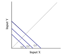
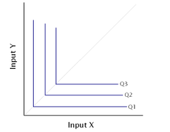
The shape of the Isoquant depends on whether inputs are substitutions or complements.

Example of an isoquant map with two inputs that are perfect substitutes.
Example of an isoquant map with two inputs that are perfect complements.

Convexity

As we always assume diminishing returns, so MRTS normally is declining. Thus, the Isoquant is convex to the origin.

However, if there is an increasing return of scale, or there is a negative elasticity of substitution ( as the ratio of input A to input B increases, the marginal product of A relative to B increases rather than decreases), then the Isoquant could be non-convex.

A nonconvex isoquant is prone to produce large and discontinuous changes in the price minimizing input mix in response to price changes. Consider for example the case where the isoquant is globally nonconvex, and the isocost curve is linear. In this case the minimum cost mix of inputs will be a corner solution, and include only one input (for example either input A or input B). The choice of which input to use will depend on the relative prices. At some critical price ratio, the optimum input mix will shift from all input A to all input B and vice versa in response to a small change in relative prices.

Reference

Learned from Wikipedia.

https://en.wikipedia.org/wiki/Isoquant

Lagrange Multiplier

Here is a review of the method of Lagrangian method. We find that maximising a utility function s.t. a budget constant by using Lagrangian could also get the MRS.

$$\max_{x,y} U(x,y)\quad s.t.\quad BC$$

Or, in a Cobb-Douglas utility.

$$\max_{x,y} x^a y^b\quad s.t.\quad p_x x+p_y y\leq w $$

Using the Lagrange Multiplier,

$$\mathcal{L}=x^a y^b +\lambda (w-p_x x- p_y y)$$

Discuss the complementary slackness, and take F.O.C.

$$ \frac{\partial \mathcal{L}}{\partial x}=0 \Rightarrow a x^{a-1}y^b=\lambda p_x $$

$$ \frac{\partial \mathcal{L}}{\partial y}=0 \Rightarrow x^a b y^{b-1}=\lambda p_y $$

Divide those two equations then we get,

$$ \frac{MU_x}{MU_y}=\frac{ay}{bx}=\frac{p_x}{p_y}=MRS_{x,y} $$

After knowing the Marshallian Demandm \(x=f(p_x,p_y,w)\), we can then calculate the elasticity.

  • \(\varepsilon=\frac{\partial x}{\partial p_x}\frac{p_x}{x}\), elasticity to price of x.
  • \(\varepsilon_I=\frac{\partial x}{\partial w}\frac{w}{x}\), elasticity to wealth.
  • \( \varepsilon_{xy}=\frac{\partial x}{\partial p_y}\frac{p_y}{x} \), elasticity to price of y.

Meaning of Lambda

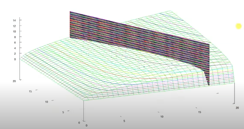
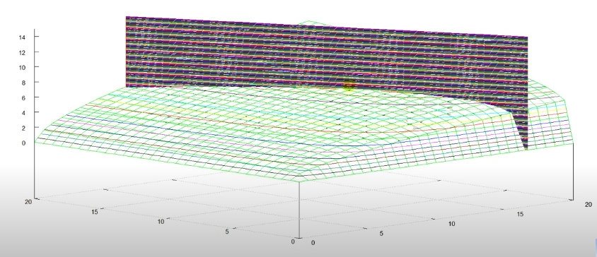
Review the graphic version of the utility maximisation problem, the budget constraint is the black plane, the utility function is green, and the value of utility is the contour of the utility function.

After solving the utility maximisation problem, we would get \(x^*\) and \(y^*\) (they have exact values). Then, plug them back into the F.O.C., we get easily get the numerical value of \(\lambda\).

As \(\frac{\partial \mathcal{L}}{\partial w}=\lambda\), \(\lambda\) represents how does the utility changes if wealth changes a unit.

\(\lambda\) is like the slope of the utility surface. With the increase, the wealth, the budget constraint (the black wall) moves outwards, and then the changes would result in an increase of the utility value, which is the intersection of the utility surface and the budget constraint surface.

Similarly, the utility function could be replaced with production and has a similar implication of output production.

Geographical Meaning

\(\lambda\) is when the gradient of the contour of the utility function is in the same direction as the gradient of constraint. Or says, the gradient of \(f\) is equal to the gradient of \(g\).

In another word, the Lagrange multiplier \(\lambda\) gives the max and min value of \(x\) and \(y\), and also the corresponding changing speed of those max or mini values of our objective function, \(f\), if the constraint, \(g\), releases.

Lagrange Multiplier:

Simultaneously solve \(\nabla f=\lambda\nabla g\), and \(g=0\). \(f\) here is the objective function (utility function in our case), and \(g\) here is the constraint (the budget constraint in our case).

Reference

Thanks to the video from Professor Burkey, that helps a lot to let me rethink the meaning of lambda.

https://www.youtube.com/watch?v=O3MFXT7AdPg

And the geographic implication of Lagrange multiplier method.

https://www.youtube.com/watch?v=8mjcnxGMwFo

MRS and MRTS

Derivations

We here derive why \(MRS_{x,y}=\frac{MU_x}{MU_y}\).

Let \(U(x,y)=f(x,y)\), and we know, by definition, MRS measures how many units of x is needed to trade y holding utility constant. Thus, we keep the utility function unchanged, \(U(x,y)=C\), and take differentiation and find \(-dy/dx\).

$$f(x,y) dx=C dx$$

$$ \frac{\partial f(x,y)}{x}+\frac{\partial f(x,y)}{\partial y}\frac{\partial y}{\partial x}=0 $$

$$\frac{\partial y}{\partial x}=-\frac{\frac{\partial f(x,y)}{\partial x}}{\frac{\partial f(x,y)}{\partial y}}=\frac{MU_x}{MU_y}$$

Therefore,

MRS_{x,y}=-\frac{dy}{dx}=\frac{MU_x}{MU_y}

$$|MRS_{x,y}|=-\frac{dy}{dx}=\frac{MU_x}{MU_y} $$

Example 1

$$U=x^2+y^2$$

$$MRS_{x,y}=\frac{MU_x}{MU_y} =\frac{x}{y}$$

Example 2

$$U=x\cdot y$$

, which is similar as the Cobb-Douglas form but has exponenets zero.

$$MRS_{x,y}=\frac{MU_x}{MU_y} =\frac{y}{x}$$

Example 3

Perfect Substitution: MRS constant
Perfect Complement

MRTS

Marginal Rate of Technical Substitution (MRTS) measures the amount of cost which a specific input can be replaced for another resource of production while maintaining a constant output.

$$MRTS_{K,L}=-\frac{\Delta K}{\Delta L}=-\frac{d K}{d L}=\frac{MP_L}{MP_K}$$

How to derive that?

Recall the Isoquant that is equivalent to the contour line of the output function. MRTS is like the slope of the isoquant line. We let,

$$Q=L^a K^b$$

Then,

$$MP_K=\frac{\partial Q}{\partial K}=b L^A K^{b-1}$$

$$MP_L=\frac{\partial Q}{\partial L}=a L^{a-1}K^b$$

$$MRTS=\frac{ b L^A K^{b-1} }{ a L^{a-1}K^b }=\frac{aK}{bL}$$

In short, MRTS is a similar concept to MRS, but in the output aspect.

Cobb-Douglas Function

Cobb-Douglas Utility function

$$U=C x^a y^b$$

While applying the Cobb-Douglas formed utility function, we are actually proxy the preference of people. (The utility function is like a math representation if individuals’ preference is rational). In the utility function, we are focusing more on the Marginal Rate of Substitution between goods.

$$MRS_{x,y}=\frac{MU_x}{MU_y}=\frac{\partial U/\partial x}{\partial U/\partial y}=\frac{Cax^{a-1}y^b}{Cx^a by^{b-1}}$$

$$MRS_{x,y}=\frac{ay}{bx}$$

P.S. Cobb-Douglas gives the same MRS to CES utility function. While solving the utility maximisation problem, we take partial derivatives to the lagrangian and then solve them. Those steps are similar to calculating the MRS.

The key is that the number or value of the utility function does not matter, but the preference represented by the utility function is more important. Any positive monotonic transformation will not change the preference, such as logarithm, square root, and multiply any positive number.

Exponents Do Not Matter

The powers of the Cobb-Douglas function does not really matter as long as they are in the “correct” ratio. For example,

$$ U_1=Cx^7y^1,\quad and \quad U_2=Cx^{7/8}y^{1/8} $$

$$MRS_1=\frac{7y}{x}\quad and \quad MRS_2=\frac{7y/8}{x/8}=\frac{7y}{x}$$

Therefore, we can find that those two utility functions represent the same preference!

Or we can write \(U_1=(U_2)^8 \cdot C^{-7}\). Both taking exponent and multiplying a positive constant are positive monotonic transformations. Therefore, the powers of Cobb-Douglas do not really matter to represent the preference. (\(U=Cx^a y^{1-a}\) the exponents of the utility function does not have to be sum to one).

$$U=x^a y^b \Leftrightarrow x^{\frac{a}{a+b}}y^{\frac{b}{a+b}}$$