Here is a review of the method of Lagrangian method. We find that maximising a utility function s.t. a budget constant by using Lagrangian could also get the MRS.
$$\max_{x,y} U(x,y)\quad s.t.\quad BC$$
Or, in a Cobb-Douglas utility.
$$\max_{x,y} x^a y^b\quad s.t.\quad p_x x+p_y y\leq w $$
Using the Lagrange Multiplier,
$$\mathcal{L}=x^a y^b +\lambda (w-p_x x- p_y y)$$
Discuss the complementary slackness, and take F.O.C.
$$ \frac{\partial \mathcal{L}}{\partial x}=0 \Rightarrow a x^{a-1}y^b=\lambda p_x $$
$$ \frac{\partial \mathcal{L}}{\partial y}=0 \Rightarrow x^a b y^{b-1}=\lambda p_y $$
Divide those two equations then we get,
$$ \frac{MU_x}{MU_y}=\frac{ay}{bx}=\frac{p_x}{p_y}=MRS_{x,y} $$
After knowing the Marshallian Demandm \(x=f(p_x,p_y,w)\), we can then calculate the elasticity.
- \(\varepsilon=\frac{\partial x}{\partial p_x}\frac{p_x}{x}\), elasticity to price of x.
- \(\varepsilon_I=\frac{\partial x}{\partial w}\frac{w}{x}\), elasticity to wealth.
- \( \varepsilon_{xy}=\frac{\partial x}{\partial p_y}\frac{p_y}{x} \), elasticity to price of y.
Meaning of Lambda

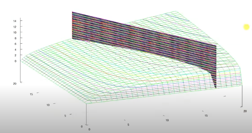
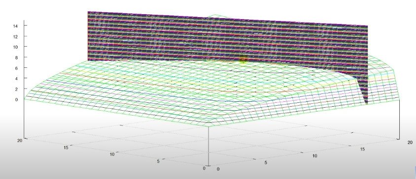
Review the graphic version of the utility maximisation problem, the budget constraint is the black plane, the utility function is green, and the value of utility is the contour of the utility function.
After solving the utility maximisation problem, we would get \(x^*\) and \(y^*\) (they have exact values). Then, plug them back into the F.O.C., we get easily get the numerical value of \(\lambda\).
As \(\frac{\partial \mathcal{L}}{\partial w}=\lambda\), \(\lambda\) represents how does the utility changes if wealth changes a unit.

\(\lambda\) is like the slope of the utility surface. With the increase, the wealth, the budget constraint (the black wall) moves outwards, and then the changes would result in an increase of the utility value, which is the intersection of the utility surface and the budget constraint surface.
Similarly, the utility function could be replaced with production and has a similar implication of output production.
Geographical Meaning
\(\lambda\) is when the gradient of the contour of the utility function is in the same direction as the gradient of constraint. Or says, the gradient of \(f\) is equal to the gradient of \(g\).
In another word, the Lagrange multiplier \(\lambda\) gives the max and min value of \(x\) and \(y\), and also the corresponding changing speed of those max or mini values of our objective function, \(f\), if the constraint, \(g\), releases.
Lagrange Multiplier:
Simultaneously solve \(\nabla f=\lambda\nabla g\), and \(g=0\). \(f\) here is the objective function (utility function in our case), and \(g\) here is the constraint (the budget constraint in our case).
Reference
Thanks to the video from Professor Burkey, that helps a lot to let me rethink the meaning of lambda.
https://www.youtube.com/watch?v=O3MFXT7AdPg
And the geographic implication of Lagrange multiplier method.