Maximum Likelihood Estimator

Joint Probability Density Function or Likelihood Function:

$f(x_1, x_2, …, x_n|\theta) = f(x_1|\theta) f(x_2|\theta) … f(x_N| \theta) $

$f(x_1, x_2, …, x_n|\theta) = \prod_{i=2}^n f(X_i | \theta) =L(\theta)$

A likelihood function is the density function regarded as a function of \theta.

$ L(\theta |x) = \prod f(x|\theta) $, $\theta \in \Theta$

As we know the sample, we need to ‘guess’ the parameter \theta to let the joint prob distribution have a maximum probability.

The Maximum Likelihood Estimator (MLE) is :

$ \hat{\theta}(x) = arg\max_{\theta} L(\theta|x) $

To simplify the calculation, we normally apply a logarithm transformation,

$$ l(\theta)= log\ L $$

$$log L(\theta |x) =log \prod f(x|\theta)= \sum_{i=1}^N log\ f_{\theta} (y_i) $$

As the logarithm transformation is monotonous,

$$ \hat{\theta}(x) = arg\max_{\theta} L(\theta|x) \Leftrightarrow $$

$$\hat{\theta}(x) = arg\max_{\theta} l(\theta|x) $$

To review it, we aim to estimate the parameters. The logic of the MLE estimator is that we guess a probability distribution, fitting into our data (sample). Then, we find or guess the value of parameters such that the joint probability function (likelihood function) achieves the maximum value.

In another word, we guess the probability dist and parameters to make sample data achieve highest possibility.

To find the argmax_{\theta} l(\theta) is equivalent to argmin_{\theta} -l(\theta)

A Normal Distribution Example

A normal distribution example,for random sample x_i, i=1, 2, 3, …, N

$$f_{\theta}(x) = \frac{1}{\sqrt{2\pi \sigma^2}}e^{-\frac{(x-\mu)^2}{2\sigma^2}} $$

We substitute f_{\theta}(x) into the log-likelihood distribution, then we find,

$$ l(\mu, \sigma^2)=log\ L(\mu,\sigma^2) $$

$$= -\frac{n}{2}\big( log2\pi + log\sigma^2 \big) -\frac{1}{2\sigma^2}\sum_{i=1}^n (x_i -\mu)^2 $$

Taking the First Order Conditions, F.O.C.

By setting \frac{\partial l}{\partial \mu}= 0 and \frac{\partial l}{\partial \sigma^2}= 0, we solve \mu_{MLE} and \sigma^2_{MLE}.

$$ \mu_{MLE} =\bar{x}$$

$$\sigma^2_{MLE} =\frac{1}{n} \sum_{i=1}^n (x_i – \bar{x})$$

P.S. We can prove that there are the local maximum, coz the second partial derivatives are negative.

def MLE_norm(x):
    mu_hat = np.mean(x)
    sigma2_hat = np.var(x)
    return mu_hat, sigma2_hat

#----------

mu = 5
sigma = 2.5
N = 10000

np.random.seed(0)
x = np.random.normal( mu, sigma, size=(N,) )

#----------

mu_hat, sigma2_hat = MLE_norm(x)

for_mu_hat = '\hat{\mu} = '+format(round(mu_hat,2))+''
for_sigma2_hat = '\hat{\sigma} = '+format(round(np.sqrt(sigma2_hat),2))+''
print('The MLE for data is:')
display(Latex(for_mu_hat))
display(Latex(for_sigma2_hat))

By our calculation, we know that mathematically the MLE estimator of mu and sigma are the mean and variance.

Perform MLE Numerically

If the log-likelihood function wasn’t continuous or differentiable. Can solve numerically through an optimisation problem where the objective function is …

In other words, sometimes we cannot calculate the MLE estimator by hand, because the log-likelihood function might not be differentiable. What can we do?

We apply the computer to interactively ‘guess’ values (Optimizer) that can end up with the maximum log-likelihood (or a minimum of negative log-likelihood).

The maximum likelihood estimator (MLE):

$$\hat{\theta}(x) = arg max_{\theta} L(\theta|x)$$

$$\hat{\theta}(x) = arg max_{\theta} L(\theta|x)$$

$$L(\theta) = \prod_{i=1}^N f(X_i | \theta) $$

$$ log\ f(X|\theta)=\sum_{i=1}^N log\ f(x_i|\theta)$$

$$ arg\max_{\theta} l(\theta) \Leftrightarrow arg\min_{\theta} -l(\theta) $$

Why we use the minimizer instead? There is only minimizer available in the scipy package, and those mini&max are basically equivalent.

def log_likelihood(theta, x):
    mu = theta[0]
    sigma = theta[1]
    l_theta = np.sum( np.log( sc.stats.norm.pdf(x, loc=mu, scale=sigma) ) )
    # there is a negative sign in front. We minimise it later.
    return -l_theta 

# Constraint Function that Restrict sigma to be positive.
def sigma_pos(theta):
    sigma = np.abs(theta[1])
    return sigma

#--------

cons_set = {'type':'ineq', 'fun': sigma_pos}

theta0 = [2,3] # inital guess. there could be any random numbers, coz it is just the intital value inputed into the optimiser
# find the minimum value of the log likelihood function
opt = sc.optimize.minimize(fun=log_likelihood, x0=theta0, args=(x,), constraints=cons_set)

for_mu_hat = '\hat{\mu} = '+format(round(opt.x[0],2))+''
for_sigma2_hat = '\hat{\sigma} = '+format(round(opt.x[1],2))+''

print('The MLE for data is:')
display(Latex(for_mu_hat))
display(Latex(for_sigma2_hat))
Kalman Filter

Definition

In statistics and control theory, Kalman filtering, also known as linear quadratic estimation (LQE), is an algorithm that uses a series of measurements observed over time, including statistical noise and other inaccuracies, and produces estimates of unknown variables that tend to be more accurate than those based on a single measurement alone, by estimating a joint probability distribution over the variables for each timeframe. The filter is named after Rudolf E. Kálmán, who was one of the primary developers of its theory.

Wikipedia

During my study in Cambridge, Professor Oliver Linton introduced the Kalman Filter in Time Series analysis, but I did not get it at that time. So, here is a revisit.

My Thinking of Kalman Filter

Kalman Filter is an algorithm that estimates optimal results from uncertain observation (e.g. Time Series Data. We know only the sample, but never know the true distribution of data or never know the true value when there are no errors).

Consider the case, I need to know my weight, but the bodyweight scale cannot give me the true value. How can I know my true weight?

Assume the bodyweight scale gives me error of 2, and my own estimate gives me error of 1. Or in another word, a weight scale is 1/3 accurate, and my own estimation is 2/3 accurate. Then, the optimal weight should be,

$$ Optimal Result = \frac{1}{3}\times Measurement + \frac{2}{3}\times Estimate $$

, where \( Measurement\) means the measurement value, and \(Estimate\) means the estimated value. We conduct the following transformation.

$$ Optimal Result = \frac{1}{3}\times Measurement +Esimate- \frac{1}{3}\times Estimate $$

Optimal Result = Esimate+\frac{1}{3}\times Measurement – \frac{1}{3}\times Estimate

Optimal Result = Esimate+\frac{1}{3}\times (Measurement – Estimate)

Therefore, we can get

Optimal Result = Esimate+\frac{p}{p+r}\times (Measurement – Estimate)

, where \(p\) is the estimation error and \(r\) is the measurement error.

For example, if the estimation error is zero, then the fraction is equal to zero. Thus, the optimal result is just the estimate.

Applying Time Series Data

$$ Optimal Result_n=\frac{1}{n}\times (meas_1+meas_2+meas_3+…+meas_{n}) $$

Optimal Result_n=\frac{1}{n}\times (meas_1+meas_2+meas_3+…+meas_{n-1})\\ +\frac{1}{n}\times meas_n

Optimal Result_n=\frac{n-1}{n}\times \frac{1}{n-1}\times (meas_1+…+meas_{n-1})\\ +\frac{1}{n}\times meas_n

Iterating the first term because\( \frac{1}{n-1}\times (meas_1+…+meas_{n-1}) = Optimal Result_{n-1} \),

Optimal Result_n=\frac{n-1}{n}\times Optimal Result_{n-1}\\ +\frac{1}{n}\times meas_n

Optimal Result_n=Optimal Result_{n-1}\\ -\frac{1}{n}\times Optimal Result_{n-1} +\frac{1}{n}\times meas_n

OResult_n=OResult_{n-1}+\frac{1}{n}\times (meas_n-OResult_{n-1})

Kalman Filter Equation

$$ \hat{x}_{n,n}=\hat{x}_{n,n-1}+K_n(z_n-\hat{x}_{n,n-1}) $$

$$ K_n=\frac{p_{n,n-1}}{p_{n.n-1}+r_n} $$

, where \(p_{n,n-1}\) is Uncertainty in Estimate, \(r_n\) is Uncertainty in Measurement, \(\hat{x}_{n,n}\) is the Optimal Estimate at \(n\), and \(z_n\) is the Measurement Value at \(n\).

The Optimal Estimate is updated by the estimate uncertainty through a Covariance Update Equation,

$$ p_{n,n}=(1-K_n)p_{n,n-1} $$

In a more intuitive way (1),

$$ OEstimate_n=OEstimate_{n-1}+K_n (meas_n-OEstimate_{n-1})$$

$$ K_n=\frac{OEstimateError_{n-1}}{OEstimateError_{n-1}+MeausreError_n}$$

$$OEstimateError_{n-1}=(1-K_{n-1})\times OEstimateError_{n-2}$$

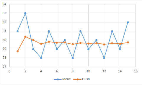
Example

numMeasMeasErrorKOEstimateOEstimateError
0755
18130.62578.751.875
28330.38461580.384621.153846
37930.277778800.833333
47830.21739179.565220.652174
58130.17857179.821430.535714
67930.15151579.696970.454545
78030.13157979.736840.394737
87830.11627979.534880.348837
98130.10416779.68750.3125
107930.0943479.622640.283019
118030.08620779.655170.258621
127830.07936579.523810.238095
138130.07352979.632350.220588
147930.06849379.589040.205479
158230.06410379.743590.192308

A Senior Study

Estimation Equation:

$$ \hat{x}_k^-=A\hat{x}_{k-1}+Bu_k $$

$$ P_k^-=AP_{k-1}A^T+Q$$

Update Equation (same as the one I just introduced in (1)):

$$K_k=\frac{P_k^- C^T}{CP_k^-C^T+R}$$

$$ \hat{x}_k^-=A\hat{x}_{k-1}+K_k(y_k-C\hat{x}_k^-) $$

$$ P_k=(1-K_kC)P_k^-$$

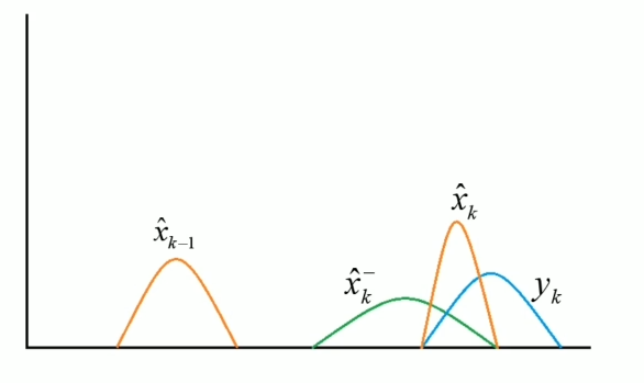
Intuitively, I need \( \hat{x}_{k-1}\) (, which is the weight last week) to calculate the optimal estimate weight this week \(\hat{x}_k\). Firstly, I estimate the weights this week \(\hat{x}_k^-\) and measure the weight this week \(y_k\). Then, combine them to get the optimal estimate weights this week.

Reading

The application of the Kalman Filter could be found in the following reading. Also, I will continue in my further study.

https://towardsdatascience.com/state-space-model-and-kalman-filter-for-time-series-prediction-basic-structural-dynamic-linear-2421d7b49fa6

Reference

https://www.kalmanfilter.net/kalman1d.html

https://www.bilibili.com/video/BV1aS4y197bT?share_source=copy_web