Definition
In statistics and control theory, Kalman filtering, also known as linear quadratic estimation (LQE), is an algorithm that uses a series of measurements observed over time, including statistical noise and other inaccuracies, and produces estimates of unknown variables that tend to be more accurate than those based on a single measurement alone, by estimating a joint probability distribution over the variables for each timeframe. The filter is named after Rudolf E. Kálmán, who was one of the primary developers of its theory.
Wikipedia
During my study in Cambridge, Professor Oliver Linton introduced the Kalman Filter in Time Series analysis, but I did not get it at that time. So, here is a revisit.
My Thinking of Kalman Filter
Kalman Filter is an algorithm that estimates optimal results from uncertain observation (e.g. Time Series Data. We know only the sample, but never know the true distribution of data or never know the true value when there are no errors).
Consider the case, I need to know my weight, but the bodyweight scale cannot give me the true value. How can I know my true weight?
Assume the bodyweight scale gives me error of 2, and my own estimate gives me error of 1. Or in another word, a weight scale is 1/3 accurate, and my own estimation is 2/3 accurate. Then, the optimal weight should be,
$$ Optimal Result = \frac{1}{3}\times Measurement + \frac{2}{3}\times Estimate $$
, where \( Measurement\) means the measurement value, and \(Estimate\) means the estimated value. We conduct the following transformation.
$$ Optimal Result = \frac{1}{3}\times Measurement +Esimate- \frac{1}{3}\times Estimate $$
Optimal Result = Esimate+\frac{1}{3}\times Measurement – \frac{1}{3}\times Estimate
Optimal Result = Esimate+\frac{1}{3}\times (Measurement – Estimate)
Therefore, we can get
Optimal Result = Esimate+\frac{p}{p+r}\times (Measurement – Estimate)
, where \(p\) is the estimation error and \(r\) is the measurement error.
For example, if the estimation error is zero, then the fraction is equal to zero. Thus, the optimal result is just the estimate.
Applying Time Series Data
$$ Optimal Result_n=\frac{1}{n}\times (meas_1+meas_2+meas_3+…+meas_{n}) $$
Optimal Result_n=\frac{1}{n}\times (meas_1+meas_2+meas_3+…+meas_{n-1})\\ +\frac{1}{n}\times meas_n
Optimal Result_n=\frac{n-1}{n}\times \frac{1}{n-1}\times (meas_1+…+meas_{n-1})\\ +\frac{1}{n}\times meas_n
Iterating the first term because\( \frac{1}{n-1}\times (meas_1+…+meas_{n-1}) = Optimal Result_{n-1} \),
Optimal Result_n=\frac{n-1}{n}\times Optimal Result_{n-1}\\ +\frac{1}{n}\times meas_n
Optimal Result_n=Optimal Result_{n-1}\\ -\frac{1}{n}\times Optimal Result_{n-1} +\frac{1}{n}\times meas_n
OResult_n=OResult_{n-1}+\frac{1}{n}\times (meas_n-OResult_{n-1})
Kalman Filter Equation
$$ \hat{x}_{n,n}=\hat{x}_{n,n-1}+K_n(z_n-\hat{x}_{n,n-1}) $$
$$ K_n=\frac{p_{n,n-1}}{p_{n.n-1}+r_n} $$
, where \(p_{n,n-1}\) is Uncertainty in Estimate, \(r_n\) is Uncertainty in Measurement, \(\hat{x}_{n,n}\) is the Optimal Estimate at \(n\), and \(z_n\) is the Measurement Value at \(n\).
The Optimal Estimate is updated by the estimate uncertainty through a Covariance Update Equation,
$$ p_{n,n}=(1-K_n)p_{n,n-1} $$
In a more intuitive way (1),
$$ OEstimate_n=OEstimate_{n-1}+K_n (meas_n-OEstimate_{n-1})$$
$$ K_n=\frac{OEstimateError_{n-1}}{OEstimateError_{n-1}+MeausreError_n}$$
$$OEstimateError_{n-1}=(1-K_{n-1})\times OEstimateError_{n-2}$$
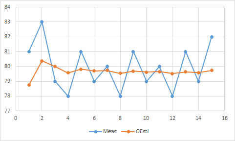
Example
| num | Meas | MeasError | K | OEstimate | OEstimateError |
| 0 | 75 | 5 | |||
| 1 | 81 | 3 | 0.625 | 78.75 | 1.875 |
| 2 | 83 | 3 | 0.384615 | 80.38462 | 1.153846 |
| 3 | 79 | 3 | 0.277778 | 80 | 0.833333 |
| 4 | 78 | 3 | 0.217391 | 79.56522 | 0.652174 |
| 5 | 81 | 3 | 0.178571 | 79.82143 | 0.535714 |
| 6 | 79 | 3 | 0.151515 | 79.69697 | 0.454545 |
| 7 | 80 | 3 | 0.131579 | 79.73684 | 0.394737 |
| 8 | 78 | 3 | 0.116279 | 79.53488 | 0.348837 |
| 9 | 81 | 3 | 0.104167 | 79.6875 | 0.3125 |
| 10 | 79 | 3 | 0.09434 | 79.62264 | 0.283019 |
| 11 | 80 | 3 | 0.086207 | 79.65517 | 0.258621 |
| 12 | 78 | 3 | 0.079365 | 79.52381 | 0.238095 |
| 13 | 81 | 3 | 0.073529 | 79.63235 | 0.220588 |
| 14 | 79 | 3 | 0.068493 | 79.58904 | 0.205479 |
| 15 | 82 | 3 | 0.064103 | 79.74359 | 0.192308 |
A Senior Study
Estimation Equation:
$$ \hat{x}_k^-=A\hat{x}_{k-1}+Bu_k $$
$$ P_k^-=AP_{k-1}A^T+Q$$
Update Equation (same as the one I just introduced in (1)):
$$K_k=\frac{P_k^- C^T}{CP_k^-C^T+R}$$
$$ \hat{x}_k^-=A\hat{x}_{k-1}+K_k(y_k-C\hat{x}_k^-) $$
$$ P_k=(1-K_kC)P_k^-$$
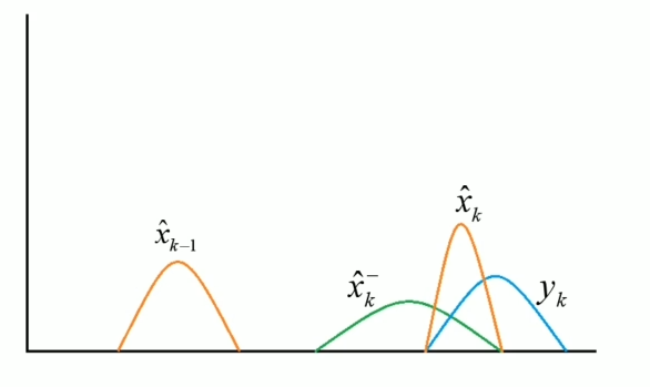
Intuitively, I need \( \hat{x}_{k-1}\) (, which is the weight last week) to calculate the optimal estimate weight this week \(\hat{x}_k\). Firstly, I estimate the weights this week \(\hat{x}_k^-\) and measure the weight this week \(y_k\). Then, combine them to get the optimal estimate weights this week.
Reading
The application of the Kalman Filter could be found in the following reading. Also, I will continue in my further study.
Reference
https://www.kalmanfilter.net/kalman1d.html
https://www.bilibili.com/video/BV1aS4y197bT?share_source=copy_web