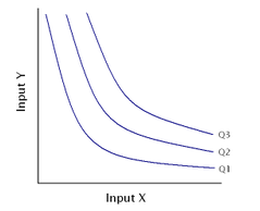
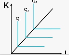
An isoquant map where production output Q3 > Q2 > Q1. Typically inputs X and Y would refer to labour and capital respectively. More of input X, input Y, or both are required to move from isoquant Q1 to Q2, or from Q2 to Q3.
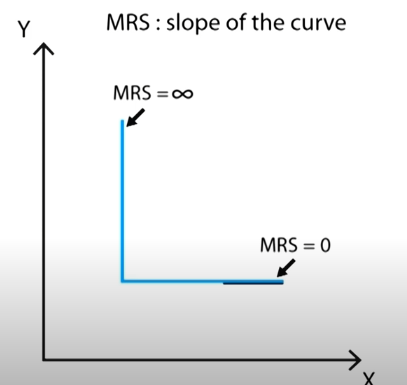
MRTS equals the slope of the Isoquant.
Difference with the Indifference Curve
Isoquant and indifference curves behave similarly, as they are all kinds of contour curves. The difference is that the Isoquant maps the output, but the indifference curve maps the utility.
In addition, the indifference curve describes only the preference of individuals but does not capture the exact value of utility. The preference is the relative desire for certain goods or services to others. However, the Isoquant can capture the exact number of production.
Shape of the Isoquant
The shape of the Isoquant depends on whether inputs are substitutions or complements.
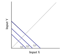
Example of an isoquant map with two inputs that are perfect substitutes.
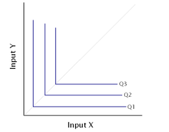
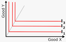
Example of an isoquant map with two inputs that are perfect complements.
Convexity
As we always assume diminishing returns, so MRTS normally is declining. Thus, the Isoquant is convex to the origin.
However, if there is an increasing return of scale, or there is a negative elasticity of substitution ( as the ratio of input A to input B increases, the marginal product of A relative to B increases rather than decreases), then the Isoquant could be non-convex.
A nonconvex isoquant is prone to produce large and discontinuous changes in the price minimizing input mix in response to price changes. Consider for example the case where the isoquant is globally nonconvex, and the isocost curve is linear. In this case the minimum cost mix of inputs will be a corner solution, and include only one input (for example either input A or input B). The choice of which input to use will depend on the relative prices. At some critical price ratio, the optimum input mix will shift from all input A to all input B and vice versa in response to a small change in relative prices.
Here is a review of the method of Lagrangian method. We find that maximising a utility function s.t. a budget constant by using Lagrangian could also get the MRS.
$$\max_{x,y} U(x,y)\quad s.t.\quad BC$$
Or, in a Cobb-Douglas utility.
$$\max_{x,y} x^a y^b\quad s.t.\quad p_x x+p_y y\leq w $$
Using the Lagrange Multiplier,
$$\mathcal{L}=x^a y^b +\lambda (w-p_x x- p_y y)$$
Discuss the complementary slackness, and take F.O.C.
$$ \frac{\partial \mathcal{L}}{\partial x}=0 \Rightarrow a x^{a-1}y^b=\lambda p_x $$
$$ \frac{\partial \mathcal{L}}{\partial y}=0 \Rightarrow x^a b y^{b-1}=\lambda p_y $$
After knowing the Marshallian Demandm \(x=f(p_x,p_y,w)\), we can then calculate the elasticity.
\(\varepsilon=\frac{\partial x}{\partial p_x}\frac{p_x}{x}\), elasticity to price of x.
\(\varepsilon_I=\frac{\partial x}{\partial w}\frac{w}{x}\), elasticity to wealth.
\( \varepsilon_{xy}=\frac{\partial x}{\partial p_y}\frac{p_y}{x} \), elasticity to price of y.
Meaning of Lambda
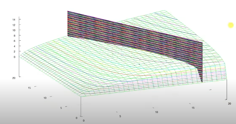
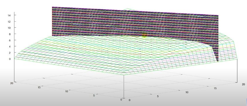
Review the graphic version of the utility maximisation problem, the budget constraint is the black plane, the utility function is green, and the value of utility is the contour of the utility function.
After solving the utility maximisation problem, we would get \(x^*\) and \(y^*\) (they have exact values). Then, plug them back into the F.O.C., we get easily get the numerical value of \(\lambda\).
As \(\frac{\partial \mathcal{L}}{\partial w}=\lambda\), \(\lambda\) represents how does the utility changes if wealth changes a unit.
\(\lambda\) is like the slope of the utility surface. With the increase, the wealth, the budget constraint (the black wall) moves outwards, and then the changes would result in an increase of the utility value, which is the intersection of the utility surface and the budget constraint surface.
Similarly, the utility function could be replaced with production and has a similar implication of output production.
Geographical Meaning
\(\lambda\) is when the gradient of the contour of the utility function is in the same direction as the gradient of constraint. Or says, the gradient of \(f\) is equal to the gradient of \(g\).
In another word, the Lagrange multiplier \(\lambda\) gives the max and min value of \(x\) and \(y\), and also the corresponding changing speed of those max or mini values of our objective function, \(f\), if the constraint, \(g\), releases.
Lagrange Multiplier:
Simultaneously solve \(\nabla f=\lambda\nabla g\), and \(g=0\). \(f\) here is the objective function (utility function in our case), and \(g\) here is the constraint (the budget constraint in our case).
Reference
Thanks to the video from Professor Burkey, that helps a lot to let me rethink the meaning of lambda.
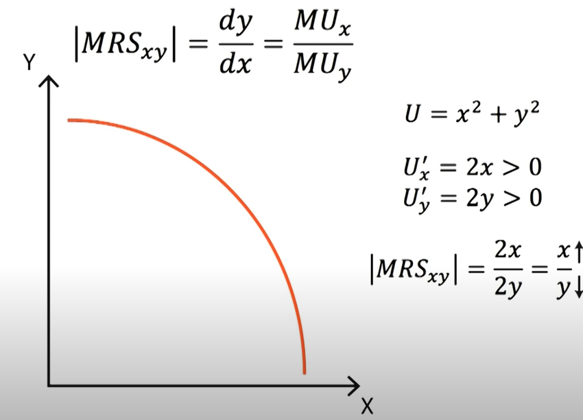
We here derive why \(MRS_{x,y}=\frac{MU_x}{MU_y}\).
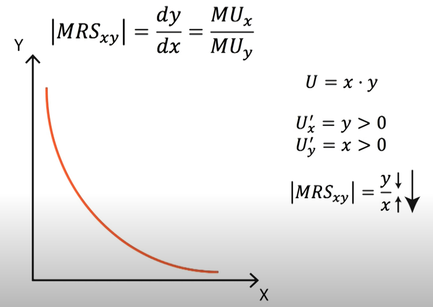
Let \(U(x,y)=f(x,y)\), and we know, by definition, MRS measures how many units of x is needed to trade y holding utility constant. Thus, we keep the utility function unchanged, \(U(x,y)=C\), and take differentiation and find \(-dy/dx\).
, which is similar as the Cobb-Douglas form but has exponenets zero.
$$MRS_{x,y}=\frac{MU_x}{MU_y} =\frac{y}{x}$$
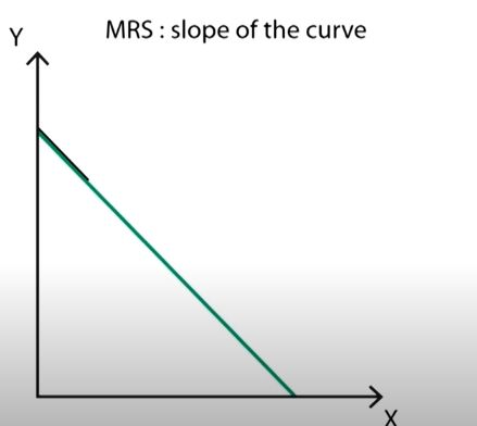
Example 3
Perfect Substitution: MRS constant
Perfect Complement
MRTS
Marginal Rate of Technical Substitution (MRTS) measures the amount of cost which a specific input can be replaced for another resource of production while maintaining a constant output.
While applying the Cobb-Douglas formed utility function, we are actually proxy the preference of people. (The utility function is like a math representation if individuals’ preference is rational). In the utility function, we are focusing more on the Marginal Rate of Substitution between goods.
P.S. Cobb-Douglas gives the same MRS to CES utility function. While solving the utility maximisation problem, we take partial derivatives to the lagrangian and then solve them. Those steps are similar to calculating the MRS.
The key is that the number or value of the utility function does not matter, but the preference represented by the utility function is more important. Any positive monotonic transformation will not change the preference, such as logarithm, square root, and multiply any positive number.
Exponents Do Not Matter
The powers of the Cobb-Douglas function does not really matter as long as they are in the “correct” ratio. For example,
$$ U_1=Cx^7y^1,\quad and \quad U_2=Cx^{7/8}y^{1/8} $$
$$MRS_1=\frac{7y}{x}\quad and \quad MRS_2=\frac{7y/8}{x/8}=\frac{7y}{x}$$
Therefore, we can find that those two utility functions represent the same preference!
Or we can write \(U_1=(U_2)^8 \cdot C^{-7}\). Both taking exponent and multiplying a positive constant are positive monotonic transformations. Therefore, the powers of Cobb-Douglas do not really matter to represent the preference. (\(U=Cx^a y^{1-a}\) the exponents of the utility function does not have to be sum to one).
CES could be either production or utility function. It provides a clear picture of how producers or consumers choose between different choices (elasticity of substitution).
CES Production
The two factor (capital, labour) CES production function was introduced by Solow and later made popular by Arrow.
Here, we get the substitution of K and L is a function of the price, w & r. As we are studying the elasticity of substitution, in other words how W/L is affected by w/r, we take derivatives later. We denote \(V=K/L\), and \(Z=w/r\). Then,
Therefore, we get the elasticity of substitution becomes constant, depending on \(\rho\). The interesting thing happens here.
If \(-1<\rho<0\), then \(\sigma>1\).
If \(0<\rho<\infty\), then \(\sigma<1\).
If \(\rho=0\), then, \(\sigma=1\).
Utility Function
Marginal Rate of Substitution (MRS) measures the substitution rate between two goods while holding the utility constant. The elasticity between X and Y could be defined as the following,
The elasticity of substitution here is defined as how easy is to substitute between inputs, x or y. In another word, the change in the ratio of the use of two goods w.r.t. the ratio of their marginal price. In the utility function case, we can apply the formula,
\(MRS_{X,Y}=\frac{dy}{dx}=\frac{U_x}{U_y}=p_x/p_y\) marginal price in equilibrium.
In the
$$ u(x,y)=(a x^{\rho}+b y^{\rho})^{1/\rho} $$
$$\sigma=\frac{1}{1-\rho}$$
If \(\rho=1\), then \(\sigma\rightarrow \infty\).
If \(\rho\rightarrow -\infty\), then \(\rho=0\).
Two common choices of CES production function are (1) Walras-Leontief-Harrod-Domar function; and (2) Cobb-Douglas function (P.S. but CES is not perfect, coz sigma always equal one).
As \(\rho=1\), the utility function would be a perfect substitute.
As \(\rho=-1\), the utility function would be pretty similar to the Cobb-Douglas form.
Later, the CES utility function could be applied to calculate the Marshallian demand function and Indirect utility function, and so on. Also, easy to show that the indirect utility function \(U(p_x,p_y,w)\) is homogenous degree of 0.
Reference
Arrow, K.J., Chenery, H.B., Minhas, B.S. and Solow, R.M., 1961. Capital-labor substitution and economic efficiency. The review of Economics and Statistics, 43(3), pp.225-250.
Definition (Homogeneity of degree \(k\)). A utility function \(u:\mathbb{r}^n\rightarrow \mathbb{R}\) is homogeneous of degree \(k\) if and only if for all \(x \in \mathbb{R}^n\) and all \(\lambda>0\), \(u(\lambda x)=\lambda^ku(x)\).
Constant Return to Scale: CRTS production function is homogenous of degree 1. IRTS is homogenous of degree \(k>1\). DRTS is homogenous of degree \(k<1\).
The Marishallian demand is homogeneous of degree zero. \(x(\lambda p,\lambda w)=x(p,w)\). (Maximise \(u(x)\) s.t. \(px<w\). “No Money Illusion”.
Excess demand is also homogeneous degree of zero. Easy to prove by the Marshallian Demand.
$$CRTS:\quad F(aK,aL)=aF(K,L) \quad a>0$$
$$IRTS:\quad F(aK,aL)>aF(K,L) \quad a>1$$
$$DRTS:\quad F(aK,aL)<aF(K,L) \quad a>1$$
2. Euler’s Theorem
Theorem (Euler’s Theorem) Let \(f(x_1,…,x_n)\) be a function that is homogeneous of degree k. Then,
Proof: Differentiate \(f(tx_1,…,tx_n)=t^k f(x_1,…,x_n)\) w.r.t \(t\) and then set \(t=1\).
P.S. We use Euler’s Theorem in the proof of the Solow Model.
3. Envelop Theorem
Motivation:
Given \(y=ax^2+bx+c, a>0, b,c \in \mathbb{R}\), we need to know how does a change in the parameter \(a\) affect the maximum value of \(y\), \(y^*\)?
We first define \(y^*=\max_{x} y= \max_{x} ax^2+bx+c \). The solution is \(x^*=-\frac{b}{2a}\), and plug it back into \(y\), we get \(y^*=f(x^*)=\frac{4ac-b^2}{4a}\). Now, we take derivative w.r.t. \(a\). \(\frac{\partial y^*}{\partial a}=\frac{b^2}{4a^2}\). We would find that,
Think of the ET as an application of the chain rule and then F.O.C., our goal is to find how does parameter affect the already maximised function \(v(q)=f(x^*(q),q)\).
A formal expression
Theorem (Envelope Theorem). Consider a constrained optimisation problem \(v(\theta)=\max_x f(x,\theta)\) such that \(g_1(x,\theta)\geq0,…,g_K(x,\theta)\geq0\).
Comparative statics on the value function are given by: (\(v(\theta)=f(x,\theta)|_{x=x^*(\theta)}=f(x^*(\theta),\theta)\))
(for Lagrangian \(\mathcal{L}(x,\theta,\lambda)\equiv f(x,\theta)+\sum_{k}\lambda_k g_k(x,\theta)\)) for all \(\theta\) such that the set of binding constraints does not change in an open neighborhood.
Roughly, the derivative of the value function is the derivative of the Lagrangian w.r.t. parameters, \(\theta\), while argmax those unknows (\(x=x^*\)).
4. Hicksian and Marshallian demand + Shepherd’s Lemma
A Taylor series is a series expansion of a function about a point. A one-dimensional Taylor series is an expansion of a real function \(f(x)\) about point \(x=a\) is given by,
, where those coefficients are free to change, and the magnitude of those coefficients would affect how the approcimated curve looks like.
To get a better approximation, we would adjust those coefficients. Thus, we consider using different orders of derivatives to simulate our target function.
We need the first order derivate of \(cos'(x)|_{x=0}=sin(x)|_{x=0}\) to be zero, so we set the first-order derivative of our polynomial function to equal to zero as well!
Let’s go one more step. As the second derivative of \(cos^{(2)}(x)=-1\), we need the second derivative (, which is also the second derivate of the second-order term of our constructed polynomial function) of our polynomial function to be also -1.
We adjust that to be negative one, so \(c_2=-\frac{1}{2}\).
Therefore, we get,
$$cos(x)|_{x=0}\approx P(x)=c_0+c_1 x +c_2 x^2 = 1-\frac{1}{2}x^2$$
Great! If we need a more accurate approximation, then we keep on going to more derivates and calculate the coefficient of the higher-order term. However, I would do that, so I just simply add a term \(O(x^3)\) to represent there are other terms that are less equal than \(x^3\). (There are accurate descriptions that I will update in later posts).
In statistics and control theory, Kalman filtering, also known as linear quadratic estimation (LQE), is an algorithm that uses a series of measurements observed over time, including statistical noise and other inaccuracies, and produces estimates of unknown variables that tend to be more accurate than those based on a single measurement alone, by estimating a joint probability distribution over the variables for each timeframe. The filter is named after Rudolf E. Kálmán, who was one of the primary developers of its theory.
Wikipedia
During my study in Cambridge, Professor Oliver Linton introduced the Kalman Filter in Time Series analysis, but I did not get it at that time. So, here is a revisit.
My Thinking of Kalman Filter
Kalman Filter is an algorithm that estimates optimal results from uncertain observation (e.g. Time Series Data. We know only the sample, but never know the true distribution of data or never know the true value when there are no errors).
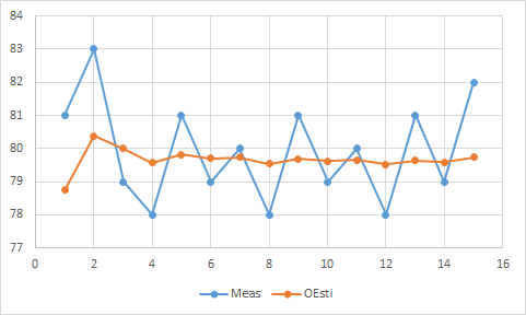
Consider the case, I need to know my weight, but the bodyweight scale cannot give me the true value. How can I know my true weight?
Assume the bodyweight scale gives me error of 2, and my own estimate gives me error of 1. Or in another word, a weight scale is 1/3 accurate, and my own estimation is 2/3 accurate. Then, the optimal weight should be,
$$ Optimal Result = \frac{1}{3}\times Measurement + \frac{2}{3}\times Estimate $$
, where \( Measurement\) means the measurement value, and \(Estimate\) means the estimated value. We conduct the following transformation.
$$ Optimal Result = \frac{1}{3}\times Measurement +Esimate- \frac{1}{3}\times Estimate $$
Optimal Result = Esimate+\frac{1}{3}\times Measurement – \frac{1}{3}\times Estimate
Optimal Result = Esimate+\frac{1}{3}\times (Measurement – Estimate)
Therefore, we can get
Optimal Result = Esimate+\frac{p}{p+r}\times (Measurement – Estimate)
, where \(p\) is the estimation error and \(r\) is the measurement error.
For example, if the estimation error is zero, then the fraction is equal to zero. Thus, the optimal result is just the estimate.
, where \(p_{n,n-1}\) is Uncertainty in Estimate, \(r_n\) is Uncertainty in Measurement, \(\hat{x}_{n,n}\) is the Optimal Estimate at \(n\), and \(z_n\) is the Measurement Value at \(n\).
The Optimal Estimate is updated by the estimate uncertainty through a Covariance Update Equation,
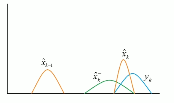
Intuitively, I need \( \hat{x}_{k-1}\) (, which is the weight last week) to calculate the optimal estimate weight this week \(\hat{x}_k\). Firstly, I estimate the weights this week \(\hat{x}_k^-\) and measure the weight this week \(y_k\). Then, combine them to get the optimal estimate weights this week.
Reading
The application of the Kalman Filter could be found in the following reading. Also, I will continue in my further study.