Insights about US Deficits and the Impact on Bond Yields
Facts
- Trump Administration is widely seen as likely to increase or maintain high fiscal deficits.
-
To assess the impact of large deficits on yields, it is important to look at the total debt in the economy,
not just government debt.What matters for markets and the economy is how much collective new credit is being created, and the incentive and desire of investors to buy it.
-
Debt Supply & Demand amount would flow to Rate. If government spending increases, then it means debt supply increases (there would be more borrowing), pushing up rate to increase.
High Borrowing -> High Rate -> Depressed the private borrowing.
Low/Normal level of credit creation would otherwise drive down inflation.
Two Cases:
-
Bad Scenario: Push up Inflation.
Total Debt/GDP increase (private and public debt / GDP) increase && Currency Weaken. Then Yield Curve would steepen, derived by long term rate increase, as nobody purchase the long term bond.
Think about a graph with x-axis (term), y-axis (yield), and a upward sloping curve.
Yield curve steepens.
-
Good Scenario (now the US situation): Do not drive up Inflation
Under this case, no buyers are buying the long-term debts.
Total Debt/GDP increases, but yield curve is flat. Public squeezes private investment. The increase in public debt does not increase private borrowing, so no extra purchasing resulted from households. Help relieve the inflation.
Yield curve flattens.
-
Example:
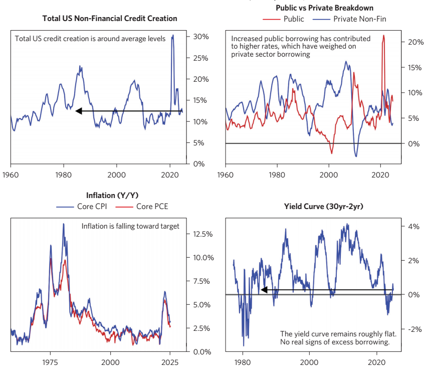
Now is the Good Scenario: The top-left figure shows the current credit creation in US is under normal level. Top-right figure shows that Public and Private debts are negative correlated. Public squeezes private, so total debt did not get up too much high.
1980s: Top-left figure shows total debts went high; Top-right figure shows public and private were positively correlated. So, bottom-left figure shows inflation hikes.
Bottom-right figure shows implicitly that the current long minus short term rate is at low level, imply that the yield curve is flat, consistent with our Good/Bad Scenario Rationale.
Supply & Supply Side of Debts
-
Supply Side: Currently, there are high public borrowing, and low private borrowing.
-
Demand Side:
Due to previous QE, Debt yield is high for investors => that would be attractive to un-levered investors, because Debts still bring enough return and less risks, attractive to people.
However, the levered investors fact different situation. As they hold debts already, high debt rate would become both their costs and returns.
-
The current real yield is about 2% in US, which is high relative to much of the rest of developed world. US nominal yields are at levels where the yield is attractive and diversifying relative to stocks allocation for those who need to supplement debts into their portfolio.

Again, the current yield curve is flat. For leveraged investors, they have debts liability already. Returns and Costs of debts offset.
Reference
Bridge-Water
Our Thoughts on Large US Deficits and Their Impact on Bond Yields
Market Timing
Allocating assets into different asset classes may depend on the (1) risk aversion, (2) time horizon, (3) tax status. And the (4) market timing also matters.
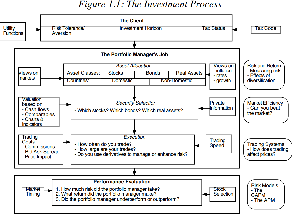
In other words, sensing the market timing would help you
- allocate assets into different asset classes such as debts, equity;
- be out of the market in the bad months, and get into the mkt in the good period.
Cost of Market Timing
- Out at the wrong time. Miss the opportunity of growth, i.e..
- Transaction Costs
- Taxes
Market Timing Approaches
Non-financial indicators
- Spurious indicators that may seem to be correlated with the market but have no rational basis.
- Though there is no reasoning, there may still have some statistical pattern. Do not ignore it.
- Those indicators give a sense of direction.
- Feel good indicators that measure how happy investors are feeling – presumably, happier individuals will bid up higher stock prices.
- The problem is that those indicators provide contemporaneous or lagging status of the market, may lack of predictability compared with the leading indicators.
- Hype indicators.
- Still the contemporaneous problem. Those factors tell the correlation right now, but do not have predictive power.
- Also, the abnormality can be tricky when the environment is shifting.
- Technical indicators, such as price charts and trading volume.
- Past prices (such as price reversals or momentum, January Indicator)
Hard to say the momentum or the reversal could stay for years.
- Trading Volume & Money Flow
-
Price increases that occur without much trading volume are viewed as less likely to carry over.
- And, very heavy trading volume can also indicate the turning points in the markets.
-
The money flow is the difference between uptick volume and downtick volume. People find there are some predictability for longer periods, in that the equity markets overall show momentum.
-
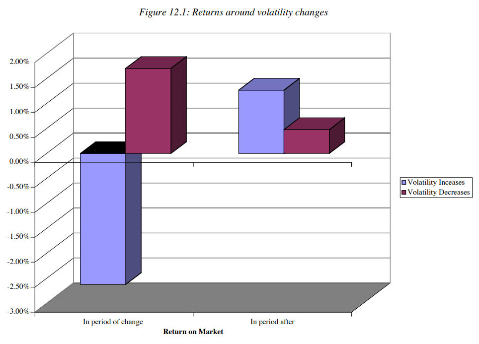
Market Volatility
-
Empirical research finds some evidence between the volatility change and returns.
-
See the blue bar: In periods that volatility increase and the market return goes down. After that period, the market is predicted to be like volatility increase and market return goes up.
-
Purple bar: in periods of volatility decrease and market return increase, the following period may have less volatility decrease and still returns.
-
Other price and sentiment indicators
-
Chart Patterns: supports and resistance lines are used to determine when to move in and out of individual stocks.
- Sentiment indicators: measure the mood of the market.
- Trader sentiments
Mean Reversion indicators, where stocks and bonds are viewed as mis-priced if they trade outside what is viewed as a normal range.
That approach is based on the assumption that stock price would revert to the P/E, and debt return would revert back certain interest rate.
- P/E (see figure below for the normal range of P/E ratio)
If stock is above or below the normal P/E, then it is overvalued or undervalued. The median is around 16.
The P/E might go abnormally high in recession, not only because (1) the stocks are overvalued, but also because (2) the earnings are dropped down during recession.

-
Rate performs similarly.
\Delta Interest Rate_t = 0.0139 – 0.1456 InterestRate_{t-1}, where R^2=0.728. Coefficients are significant.
The regression suggest two things:
- Change in interest rates in the period is negatively correlated with the level of rates at the end of each prior year.
- The speed shrinks. For every 1% increase in the level of current rate, the expected drop in interest rate in the next periods increases by 0.1456%.
Fundamentals
Using the fundamentals to predict market timing is to focus on macroeconomic variables such as interest rate, inflation and GNP growth and devise investing rules based upon the levels or changes in macro economic variables.
Two keys of using this approach. (to build up the logic chain of prediction)
- Get handle how the market reacts as macro econ fundamentals change.
- Get good predictions of changes in macro econ fundamentals.
- Macro economic variables, such as the level of interest rate or the state of the econ cycle.
There are some common sense that the following changes would indicate the increase in stock price:
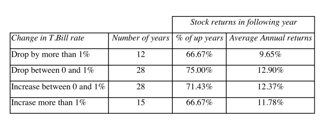
- Buy when Treasury bill rates are low, will end up with growth of stock price.
- Buy when Treasury bond rates have dropped, will end up with growth of stock price.
- Buy GNP growth is strong, will end up with growth of stock price.
However, empirical evidence shows the other way. For example, the table below shows T-bill rate drops or increases could both contribute to the increase in Annual returns.
Valuing the Market
Just as you can value individual stocks with intrinsic valuation (DCF) models and relative valuation (multiples) models, you can value the market as well. If the valuation is faithful, you can reply on it to predict the market timing.
- Intrinsic valuation that apply to the mkt. <- depends on assumptions and inputs.
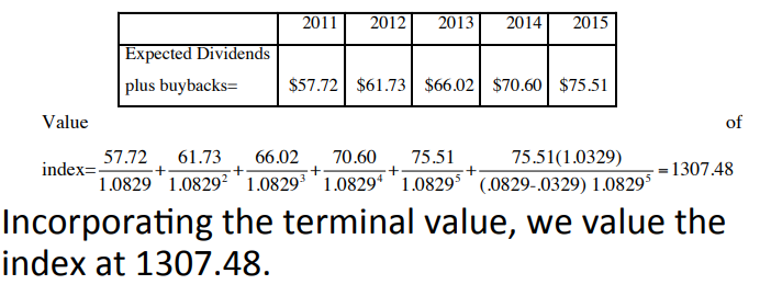
Use the S&P500 price and the index’s dividends to do the DCF.
INPUTs: (1) S&P500 price, 1257.64 at 2011(2) Dividends and buyback on the index amount over previous year, 53.96 (3) expected earning growth for the following 5 years, 6.95% (4) expected growth of the economy (set as risk free rate) 3.29%, (5) treasury bond rate, plus the market risk premium (set it yourself) 5% to get the cost of equity 3.29%+5%=8.29%. Then, do the DCF
-
Relative Valuation <- value a market relative to other market, or across years.
-
Other methods, such as run regression on P/E to T-bill to find correlation.
Does the Market Timing Work?
-
Mutual Fund Managers: constantly try to time the markets by changing the amount of cash that they hold in the fund. If expected bullish, then cash balances decreases, vice versa.
They call timing the market as Tactical Asset Allocation, TAA.
See figure below, empirical evidence shows they do predict the market by changing the cash position.

-
Investment Newsletter: often take bullish or bearish view about the market.
There is continuity on Newsletter way. Investment newsletters that give bad advice on market timing are more likely to continue to give bad advice than are newsletters that gave good advice to continue giving good advice. In other words, it depend on the writer’s ability.
-
Market strategists: make forecast for the overall market.
-
Professor Market Timers provide advice, however, their decision works for very short time, and only work for private clients.
Market Timing Strategies
- Adjust Asset Allocation: change across asset classes
- Switch Investment Styles: change within asset classes but different styles, such as from growth to value.
- Sector Rotation: with in asset classes, but different sector.
- Market Speculation.
Market Timing Instruments
- Futures Contracts
- Options Contracts
- ETFs
Implications and Insights
Overall, it’s good summary and a Beginner’s Tutorial, but not include technical implementation method, instruction, or philosophy.
Do provide some inspirations.
Reference
https://pages.stern.nyu.edu/~adamodar/New_Home_Page/webcastinvphil.htm
债券的分析框架
债券利率波动存在上下限区间
- 上限:实体部门的投资回报率,ROIC (return on invested capital)。因为上市公司ROIC要超过债券的利率,企业才有可能借债,不然承担不了利息成本
- 行业的负债水平与ROIC呈负相关,因为负债越高,投资回报率倾向于越低
- 高负债行业对债券市场影响大,因为规模大。
- 下限:刚性融资需求的利率水平,主要包括:城投 & 地产
- 城投代表地方政府的隐性担保,相当于信用高,风险低,因此利率低。
- 刚需融资需求萎缩,会拉低利率,因此利率下限降低
当前债券市场的特征
长短期利率脱钩,当前处于bull flat的情况
- Bull Flat 意味着:长期利率降低,长期债价格上升,短期相对不变,整个收益率曲线goes flatter
- Theoretically, 短端利率的波动大,且响应速度快。但当前短期利率没有明显变化,意味着市场对短期政策力度预期低,因此不投向短期。
后续债券市场的展望
- 方向(按照2025年利率上下限变动趋势来预测2025年利率的变动)
上限:拆分ROIC贡献的主要行业,2024年为光伏和电力等,2025年预计两行业增长有限,得有新兴产业才能支撑ROIC增长。ROIC预期不提升,因为没有增长机会;
下限:此前有刚性融资需求的城投债 & 地产拉跨,需求少,需要有新的刚性融资需求的部门增加才能推动利率下限上升。当前城投债预期也不提升,因为没有新的基建项目和空间,房地产也拉跨,因此没有需求。
总之,若无新的增长点,上下限方向均向下。
-
空间
-
当下房租(租金回报率)和按揭还款(融资成本)倒挂明显。未来有趋近的空间,因此有余地。
-
假设明年CPI回到1.5%,PPI回到0%,用贷款利率减去CPI和PPI的均值为实际利率。用此实际利率与历史对比,也仅处于中性水平。画外音,明年CPI大概率回不到1.5%,可能更低,因此明年实际利率更高,无法刺激经济。所以还有更多的降息空间。
- 此外,今年存贷款利率下调幅度多于货币市场资金成本(货币市场投资or理财收益更高),所以存款从银行表内向外转移。因为货币市场投资主要投向债等,这意味着短期债的收益高于存款利率,因此CB还有执行Open Market Operation,降息的空间。
- 节奏
-
利率走势和很多宏观指标脱钩,因为宏观统计数据失真(高估),无法反应真实情况,而利率作为市场真正交易的产品,能更好的反映市场的真实情况,因此存在利率与其他指标脱钩的情况。
-
目前,还有一个指标,企业信贷规模变化,与利率还有显著的相关性。因此可以通过推断企业信贷的供求端,即信贷供给&企业杠杆率,来推断利率变化的节奏。
-
化债or信用的周期:第一阶段,通过密集的发行新债券,置换旧债券,拉动社融增速,因为有新债券发行,对资金需求高,短期利率推高;第二阶段,逐步偿还新债券,在债务偿还过程中,信贷会收缩,利率逐步下降;第三阶段,债还接近尾声期,信贷增速和杠杆率将降到低位,利率降至低点。后续才会重启宽信用的周期。
目前还处于第一阶段,新债券集中发行会推高利率。
即使目前经济政策是降利率,但是与信贷周期短期推高利率叠加,可能导致2025年上半年(化债or信用周期的第一阶段),整体利率下降不明显,因为政策的降利率和信贷周期的升利率对冲了一部分。后半年利率会逐步下行。
但具体也要看OMO的力度。
Be careful if they Talked the Talk, Walked the walk, disappointing the mkt and people again and again.
Reference
https://www.bilibili.com/video/BV16ViRYJEY8/
关于中国经济现在 – 付鹏在汇丰的报告
当前经济模式从增长转为分配
当前经济模式由增长(把蛋糕做大),变为分配(把蛋糕切好)。参考日本的1980s后的状况,经济没有增长并不意味人均变差了或者人不幸福了(日本消失的40年),同时而经济增长也不意味着人均都增长了(近年我国的增长模式)。
如何应对
当前上述由增长转为分配的背景下,普通人需要做的是,参与到到分蛋糕的过程中,参与分配,而不是参与增长。But how to do it?
- 离权力近一点,离资源近一点,就能多吃一点。
- 而卖劳动力(按以前增长的模式挣钱),就只能少吃一点。
日本低利率时代,巴菲特carry trade,在日本发日元债,以低利率(低成本)借钱,然后直接投资日本公司。In other words, 巴菲特参与了日本过去40年的存量财富分配。
当前经济困境
经济流转的过程,一方的消费是另一方的收入。然而消费和收入流转需要时间。
- 当经济扩张时:富人先进五星级酒店,富人先买超跑,富人先吃海鲜,然后逐步下沉,到最后是老百姓吃上海鲜,老百姓开上汽车,老百姓进五星级酒店。
- 当经济收缩时,却是相反的:先收缩的是底层。网约车司机、快递员、外卖小哥等是对经济需求反馈最快的。而坐办公室的往往反馈很慢,要等年终降薪、发不出工资、裁员等才会有反馈。同时,近年网约车司机数量剧增并不是因为农村劳动力进城,更多的是,中产阶级的陨落。只不过是你的阶层不一样,你看的问题不一样。
- 从经济数据反馈,经济收缩的时候是底层先吃苦,往往一定周期后才能传递到经济数据上,因此宏观经济指标的反馈将滞后。
经济数据不真实,实际情况是通缩,没有增长。
主要原因是人口问题,老龄化及劳动人口缩减。
刺激经济的方式
关于说法“内债不是债”。诚然不同于外债需要用外汇还,有本币的国家可以通过印钱来还债,但是长期以往会导致流通中的货币增加,产生潜在通胀问题(可能当前短期通缩,因为没有过量现金流通,但货币总量增加了,长期一定会有通胀风险)。
国家政府需要长期稳定就需要保持Public Sector的平衡。债务增加需要靠(1)借新还旧(2)提升税收还。
- 税收收入 = 税基 * 税率
- 税基 = f(人口,收入,消费意向, etc)
- 税收收入 = f(人口,收入) * 税率
- 当前总人口少了,只有增加收入,或者增加税率,才能满足债务增加。
此前,公共部门的债,企业债,可以通过供给侧改革&房地产等方式输出给私人部门,换句话说是将企业和政府债转移,由老百姓买单。但当前,人口结构和人口总量不一样了。当前供给过剩,及需求不足同时存在,导致价格(PPI,CPI)一降再降。
房地产市场
房价在2008年-2015年第一波上涨,而2015年-19年才是上涨幅度最大的,此阶段也是80s后需求最旺盛的年代。然而收入增长并没有房价增长快,房价是由需求推动的,而非购买力。北京的房价收入比是世界最高的一批。
买房的时候抵押贷款,相当于把自己的未来收入折现抵押给银行,买房。房子此后换手,如200万买了卖400万,相当于把债务转移给接手人,由其未来现金流折现来偿还。所以房价上涨,而收入未上涨,相当于掏空年轻人或者中年人更多年的未来收入。
如果收入不增长,那么实际各种交易都是在做资源分配,而非增长。一批人的财富来自于另一批人的债务,如上文200万房卖400万的例子。但如果没有更多的年轻人愿意买房了,400万的房卖出600万了,相当于旁氏骗局的链条断了,比较收入没有实际增长。
而房价在整个经济体中有着重要的意义,关联着抵押和债务。如果房价降,相当于资产降,而债务不变,只能equity降低(相当于wealth降低),如果equity降到0或为负,则资不抵债。
放大到宏观,纵向,收入上涨才能保证房地产的需求和价格。而收入可以理解为未来现金流折现,未来年轻人的收入折现。如果年轻人少了,相当于能折现的收入少了,房价难免下跌。年轻人把房子买走了,让中老年或者少数人(如房地产开发)获得了财富,但是年轻人获得了负债。
未来消费结构
当前人口少了,人口结构变了,老年人成为了消费的主导(尹瑞哲的报告,年轻人少的省份消费能力强),同时中长期看,消费的结构向年轻人的方向转变
中国企业周期
中国可以用很短的时间将产业链做到“全球遥遥领先”,在政策的保护期,PPI为正,企业都可以活,但同时由于有利润空间,企业进入市场,会造成很多同类竞争。但一旦保护期一到,到市场经济竞争的情况下,企业开始打价格战,开始PK、竞争、内卷,PPI开始转负。然后一轮产业过剩,开始淘汰。
政府驱动再引导新的产业。用这种前浪推后浪的方式,推动整个产业各个环节的周期缩短到五年,但是代价就是很多行业会以很快的速度进入到PPI为负,而所有能到PPI为负的产业,最后能活下来都得感谢有自己的负债端,有居民部门能买单。一旦内需不足,居民部门不再为企业负债买单(或者无法买单,因为经济压力自底层向上传导),就会出危机,就是当前经济现状。
所以看产业链成熟度,或者说看周期投资时,不能等产业已进入竞争模式的时候投(如新能源),因为在价格战,博弈分蛋糕,就像抽签众多企业中能成活的一个(当然也不要买行业ETF,而如果一定要投此行业,投最有机会活下来的,负债端压力小的,有打价格战空间的)。要在政策利好的时候投,因为在把蛋糕做大,有政策保护。
投资是看预期,不是现状。
供给侧改革
中国供给侧改革的起点是2002年,PPI为正,核心CPI为正,有效需求为正。持续到2012年,供给开始过剩,但有效需求可以继续加杠杆(相当于居民部门用负债端扩大的方式支撑供给侧扩张),但供给矛盾已经产生,2009年供需双落,这就是中国这一轮从2012年开始的大周期的末端。
此处时间有点混乱,付鹏建议看《朱镕基总理答记者问》,三卷本。
“只要人还在,啥债都能化”。只要人不在,这债怎么化?税率。量收不上来,就抓率。
财政、利率、汇率传导
当财政需要扩张,利率下降,财政花钱短期内不会流转到居民部门,国内经济的有效需求不够,储蓄过剩,投资回报率下降,利率下降。
在这种背景下,汇率就代表着你的实际回报率以及本币购买力,是减弱的,本币贬值。
日本长期低利率,而同时保证汇率稳定的原因。理论上将,利率差会导致汇率差,但日元此前相对稳定。原因是日本进行carry trade,大企业(三井、三菱etc)低息借日元然后买海外资产。用海外资产来支撑日元汇率。然而企业通过carry trade挣了钱,老百姓无法进行此操作(其实老百姓也可以买海外股票,但是大多数老百姓没有这么做),老百姓穷了(收入降低无法支撑消费)所以日元的稳定才难以维持。
Implications
当前两会提出财政和货币双重宽松,希推高国内CPI避免通缩,短期市场可能会利好,因为投资者不希望踏空,且不希望被通胀影响。但交易上可能只有短期影响,因为债务需要用税收买单,宏观经济的核心问题(人口)并没有解决,且没有新的技术能推动经济增长,那么中长期就难以维系。
交易上可能短期实现收益后投资海外资产比较好。
Others
- 投资方向,中产面临巨大困境,做高端(爱马仕),做低端(拼多多。放弃中端(LV,Chanel,Prada)
- 消费模式类似,只有老人的消费和年轻人的消费可以做,中年人的消费能力降低。
- 投资产业要投早期的产业,已经成熟的只能投负债端优秀的或有价格战能力的。
Reference
https://www.wenxuecity.com/news/2024/12/02/125897172.html
The Fine Art of Small Talk
by Debra Fine
A book that teach you how to overcome the fear of start a conversation, and how to delicately continue the talk, making others comfortable.
1. What’s the Big Deal about Small Talk
We become better conversationalists when we employ two primary objectives.
- Take the risk, starting a conversation with a stranger.
- Assume the burden. It’s our responsibility to come up with topics to discuss, to remember people’s name and to introduce them to others, to relive the awkward moments or fill the pregnant pause.
2. Get over Your Mum’s Good Intentions.
- In safe situations, make it a point to talk to strangers. Start it!
To expand your circle of friends and colleagues, you must start engaging strangers and acquaintances in conversation. There is no other way. Strangers have the potential to become good friends, long-term clients, valued associates, and bridges to new experiences and other people. Start thinking of strangers as people who can bring new dimensions to your life, not as persons to be feared.
-
Introduce yourself.
People expect you to mingle on your own, introduce yourself, and take the initiative to get acquainted.
-
Silence is impolite
Start to talk, silence is not golden.
Don’t risk being taken as haughty or pretentious by keeping silent; it can cost you dearly. Start small talking and let others see your personality. You know how much you appreciate the efforts others put forth in conversation. Make the same effort. Contrary to what your elders taught you, silence is not golden.
-
Good things come to those who go get them!
Don’t spend another minute thinking that if you just keep waiting, interesting people will introduce themselves.
We end up paying twenty pounds to attend an event and then seek out people we already know because it’s less threatening. Yet the purpose of the event was to make new contracts.
-
It’s up to you to start a conversation
When you walk into a luncheon or a cocktail party, more people there are scared to death to talk to you. Fear of rejection keeps many of us from risking conversation, but the probability of rejection is actually quite small.
You will be the hero if you start the conversation. You will gain stature, respect, and rapport if you can get the conversation going.
-
It’s up to you to assume the burden of conversation
You cannot rely on the other person to carry the conversation for you. One-word answers to questions do not count as shouldering your share of the burden.
To become a great conversationalist becoming invested in the conversation and actively working to help the other person feel comfortable.
Ask icebreaker questions. Such as “What do you do for a living?”
3. Take the plunge: Start a conversation!
When someone gives you a smile, you are naturally inclined to smile back. Be the first to smile and greet another person. Just a smile and a few words, and it’s done. Be sure that you make eye contact. That simple act is the beginning of establishing rapport.
Mingle with the people in the audience, making a personal connection with as many as possible.
The best way to get people comfortable enough to open up and express themselves was to look them in the eye and ask “What’s your name?” Making eye contact and placing the emphasis on the word your, rather than the word “name”, signaled to the person that they were important.
- What’s in a name?
Learning and using names is probably the single most important rule of good conversation.
Focus on the name, repeat it, and then formulate your answer.
Don’t go through the while conversation pretending you know the person’s name. Say something like “Excuse me, I’m not sure I got your name”. It’s always preferable to have the other party repeat it than to fake it. Never, ever fake it!
Individuals with foreign or unusual names get slighted more than the rest of us. Make it a point to learn the proper pronunciation, even if it means that the other person repeats it a few times.
Learning names is part of hosting the conversation. A host is always expected to know and use every person’s name, since the host is responsible for making introductions as new individuals enter the conversation.
Acting as the host puts everyone at ease and creates an atmosphere of warmth and appreciation that naturally encourages conversation. It also positions you as a leader in the group.
-
It’s better to give than to receive.
Give your name when you meet someone. Extend your hand. “Hi XX. Fanyu Zhao. How are you?” By stating my name.
4. Keep the conversation going!
Instead of sitting back and waiting for another kind soul to start a conversation, take the lead. Try to make your guest as comfortable as possible.
The approachable person is the one who makes eye contact with you and who is not actively engaged in a conversation or another activity such as reading a newspaper or working at a computer.
Not only are icebreakers a good way to start conversation, but some of the statements are accompanied by questions you can ask to keep the ball rolling. Don’t use a statement alone. Using a statement by itself is like lobbing the conversational ball blindfolded, not knowing where it will land or whether it will get tossed back.
- Tips for Starting with a Conversation
- What a beautiful day. What’s your favorite season of the year?
- I was truly touched by that movie. How did you like it? Why?
- This is a wonderful restaurant. What is your favorite restaurant? Why?
- What a great conference! Tell me about the sessions you attended.
- I was absent last week. What did I miss?
- That was an interesting program after lunch. What did you think?
- Presidential campaigns seem to start immediately after the inauguration. What do you think of the campaign process?
- I am so frustrated with getting this business off the ground. Do you have any ideas?
- • I am excited about our new mayor. How do you think her administration will be different from her predecessor’s?
- Your lawn always looks so green. What is your secret?
- We’ve been working together for months now. I’d like to get to know you better. Tell me about some of your outside interests.
- You worked pretty hard on that stair stepper. What other equipment do you use?
- You always wear such attractive clothes. What are your favorite stores?
- What a beautiful home. How do you manage to run a house with four children?
- I read in the newspaper that our governor has taken another trip overseas. What do you think of all his travel?
- Easy Openers: You will be successful if you just take the initiative and give it a try. You’ll be surprised by how easy it is and at the positive reinforcement you get from people when you start a conversation. Remember the following four steps and you are well on your way to an excellent chat.
- Make eye contact.
- Smile.
- Find that approachable person!
- Offer your name and use theirs.
- Break into a group of five conversation:
- Show interest in the speaker, but stand slightly away from the group. A group this size is slow to warm, so first let them become accustomed to seeing you. Slowly, they will shift to bring you into the circle.
- Ease into the group by demonstrating that you’ve been listening. Look for welcoming signs such as them asking your opinion or physically shifting positions to better include you.
- Initially, it is best to find a point of agreement; barring that, just acknowledge the speaker. Wait before rocking the boat with a big wave of radical opinions. Before offering your views, let the group warm to you. If you come on too strong too fast, the group will resent your intrusion and disband. Then you have to start all over again, looking to chat with someone you haven’t just offended!
5. Let’s Give ’Em Something to Talk About
Your mission is to get your conversation partners talking about themselves. Most people enjoy the opportunity to share their stories, and if you give them the chance, they’ll start talking. This is a no-brainer route to small talking success.
- Asking.
By asking open-ended questions, you offer your conversation partner the opportunity to disclose as much or as little as she wants. These questions demand more than a simple yes or no answer, yet they make no stressful demands.
-
Digging Deeper
After asking the greeting type question such as “How are you?”, follow up with deep question.
These everyday inquiries are just a few other ways of saying hello. It’s almost universally understood that these questions are a form of greeting, not a sincere inquiry.
Digging in deeper indicates you truly desire a response and are prepared to invest time in hearing the response.
Dig in deeper based on your observation.
6. Hearing Aids and Listening Devices
Scientific research has shown that people are capable of listening to approximately 300 words per minute. On the flip side, most of us can only speak at 150 to 200 words per minute.
The dilemma is that we have the capacity to take in much more information than one person can divulge at any given time.
Attentive listening has three parts: visual, verbal, and mental. Combine these elements, and powerful listening results.
- Listening is seen, not just heard
Listening is more than just hearing. In a normal two-person conversation, verbal components carry less than 35% of the social meaning of the situation, while nonverbal components account for over 65%. It’s critical to maintain eye contact when you are listening to another person.
Gestures show what the counterpart’s attitude.
-
Verbalise your listening
There are numerous verbal cues to let the speaker know you are fully engaged in the conversation. These brief comments tell the speaker that you are interested and want to know more. You can use verbal cues to show that you have a positive response, that you disagree, or that you want to hear more about something in particular.
| If you want to show that you are: | Say: |
|---|---|
| Interested in hearing more … | Tell me more. What was that like for you? |
| Taking it all in… | Hmmm, I see … |
| Responding positively… | How interesting! What an accomplishment! |
| Diverging… | On the other hand, what do you think … ? |
| Expanding on the idea… | Along that same line, do you … ? Why? |
| Arguing/refuting… | What proof do you have of that? |
| Involving yourself … | Could I do that? What would it mean to me? |
| Clarifying … | I’m not sure I’m clear on your feelings about… |
| Empathising… | That must have been tough/frustrating, et cetera. |
| Probing… | What do you mean by that? How were you able to manage? |
| Seeking specifics… | Can you give me an example? |
| Seeking generalities… | What’s the big picture here? |
| Looking to the future… | What do you think will happen next? |
| Reviewing the past… | What happened first? |
| Seeking likenesses / differences | Have you ever seen anything like this? What’s the opposing point of view? |
| Seeking extremes / contrasts | What’s the downside? / What’s the optimum? |
Other verbal listening cues function to redirect the conversation by transitioning to another topic. Examples of cues that offer a seamless segue include:
- That reminds me of…
- I’ve always wanted to ask you…
- I thought of you when I heard…
- Do you mind if I change the subject?
- There’s something I’ve wanted to ask of someone with your expertise.
All these verbal cues indicate that you are fully present. Just as important, these cues encourage others to continue speaking. Imagine someone asks you a question, and you respond with a one-sentence answer. You are uncertain as to how much information they are truly interested in learning. Added verbal cues as you respond assure you that their interest is sincere.
- Tips for Tip-Top Listening
- Learn to want to listen. You must have the desire, interest, concentration, and self-discipline.
- To be a good listener, give verbal and visual cues that you are listening.
- Anticipate excellence. We get good information more often when we expect it.
- Become a **“whole body” listener: Listen with your ears, your eyes, and your heart. **
- Take notes. They aid retention.
- Listen now, report later. Plan to tell someone what you heard, and you will remember it better.
- Build rapport by pacing the speaker. Approximate the speaker’s gestures, facial expressions, and voice patterns to create comfortable communication.
- Control internal and external distractions.
- Generously give the gift of listening.
- Be present, watch the tendency to daydream. Don’t drift off from conversations.
7. Prevent Pregnant Pauses with Preparation
- Do not let old acquaintances be forgotten
Seek out what’s new and keep the conversation rolling with questions. Like…
- Bring me up to date on . . .
- What’s been going on with work since I last saw
you? - What has changed in your life since we spoke last?
- How’s your year been?
But do not ask about other’s wife / jobs / children, if you do not know the person well
-
Preparing for the long haul
When there is nothing to talk about! Here are
some examples of interviewing questions you can customise to fit your own personality: (the book gives the following examples)- What do you enjoy most about this season of the year?
- What got you involved in this organisation/event?
- If you weren’t here, what would you be doing at this very moment?
- If you could meet any one person, whom would you choose?
- Tell me about an issue that matters a great deal to you.
- What has been your most important work experience?
- Limelight Etiquette
First, disclose information about yourself that is comfortable and uncontroversial. Lead with easy, positive, and light information. Building trust and intimacy over time creates friendships. Having a conversation is a little like peeling an onion—you want to proceed in layers, matching the level of intimacy shared by your partner.
You aren’t limited to talking about events and experiences. You can share feelings, opinions about books you’ve read, restaurants you’ve visited, and movies you’ve seen.
Speak no evil: Barring exceptional circumstances, avoid these often controversial topics that can stop a conversation in its tracks:
- Stories of questionable taste
- Gossip
- Personal misfortunes, particularly current ones
- How much things cost!
- Controversial subjects when you don’t know where people stand
- Health (yours or theirs). The exception is when you’re talking with a person who has an obvious new cast, crutches, or bandage. In that situation, the apparent temporary medical apparatus is free information. If you skirt the issue, it’s a bit like having an elephant in your living room and ignoring it.
When in doubt, leave it out. Avoid any area that is likely to offend your conversation partner
Conversation Clout
-
Can you spell your name for me? Most of us know how to spell our names, we do not need to be asked first if we know how!
Instead: Please spell your name for me.
-
If I can find out … A low expectation is established when you use the word if. Raise expectations. Instill confidence.
Instead: I will look into this and get back to you one way or the other.
-
I’m only the… Everyone’s role or job is important. This is demeaning to oneself. Define the capabilities and responsibilities in
your area of expertise.Instead: My responsibilities are focused on Website development. I will be glad to check with sales about your order.
-
I can’t meet with you this morning. This projects an unwillingness to deliver the best possible outcome. Or it projects a burden. In either
case say what you can do, not what you cannot.Instead: I can be there by three this afternoon.
-
I’ll try to get this back to you this week. The word try conveys the underlying message that this is not something that is dependable.
Instead: I’ll get to you no later than next week.
Tell people what you will do, not what you hope to do. -
You’ll have to call me tomorrow. This is a busy time for me. This sounds like a person giving orders and placing another burden on my already heavy load! And I don’t like to be bossed around.
Instead: *You can call me tomorrow. That’s a better time for me.
No say no, but say what you can.
9. Crimes and Misdemeanours
-
Don’t be interpreter.
Do not interpret. The interrupter is
characterised by high drive, determination to make her point, and a lack of patience.There are only three good reasons for interrupting. The first is that you need to exit immediately. The second is that the topic of conversation is too uncomfortable to bear, and you need to change the subject right away. And the third is if you are in the company of a monopoliser who has refused to offer you a natural break in the conversation for more than five minutes.
10. The Graceful Exit
There are ways to artfully exit a conversation that leave the other person’s ego intact. I find that many people remain in a conversation longer than they should for two reasons: they feel trapped, especially if it’s just a two-person dialogue, or they are so comfortable that they don’t want to leave.
- When you prepare to depart a conversation, recall why you originally connected with your conversation partner and bring the conversation back to that topic.
For example:
Tom, (1) it’s been wonderful talking with you about the changes impacting the health-care industry. (2) I need to catch up with another client before she leaves. (3) Thanks for sharing your expertise.
Notice that the author didn’t make excuses for my leaving. The author didn’t say I had to call the babysitter or that I needed to return a page. That well-known adage “honesty is the best policy”
You clearly state that the reason you are leaving the conversation is that you need to do something. There is no mistaking the fact that you have a specific agenda that you are trying to accomplish.
-
A Little Appreciation goes a long way
Ending a conversation by showing appreciation for the interchange provides an upbeat way to leave on a positive note. Thanking others for their time, expertise, or the sheer joy of the conversation is always welcome.
Remember to end the conversation the same way you began it—with a smile and a handshake. Even if you have to get up and walk around the table to do this, make sure you do. You make a lasting impression when you seal a conversation with a handshake.
-
Parting is such sweet sorrow
If you’ve met someone with whom you’d like to further a relationship, the best way to exit is to ask to see him again.
11. The conversational Ball is in your court!
A cheat sheet of tips here. Take the risk and assume the burden, and do start to talk.
Fifty Ways to Fuel a Conversation
- Be the first to say hello.
- Introduce yourself to others.
- Take risks and anticipate success.
- Remember your sense of humour.
- Practice different ways of starting a conversation.
- Make an extra effort to remember people’s names.
- Ask a person’s name if you’ve forgotten it.
- Show curiosity and sincere interest in finding out about others.
- Tell others about the important events in your life. Don’t wait for them to draw it out.
- Demonstrate that you are listening by restating their comments in another way.
- Communicate enthusiasm and excitement about your subjects and life in general.
- Go out of your way to try to meet new people wherever you are.
- Accept a person’s right to be an individual with different ideas and beliefs.
- Let the natural person in you come out when talking with others.
- Be able to succinctly tell others—in a few short sentences—what you do.
- Reintroduce yourself to someone who is likely to have forgotten your name.
- Be ready to tell others something interesting or challenging about what you do.
- Be aware of open and closed body language.
- Smile, make eye contact, offer a handshake, and go find the approachable person.
- Greet people that you see regularly.
- Seek common interests, goals, and experiences with the people you meet.
- Make an effort to help people if you can.
- Let others play the expert.
- Be open to answering common ritualistic questions.
- Be enthusiastic about other people’s interests.
- See that the time is balanced between giving and receiving information.
- Be able to speak about a variety of topics and subjects.
- Keep up to date on current events and issues that affect our lives.
- Be willing to express your feelings, opinions, and emotions to others.
- Use “I” when you speak about your own feelings and personal things, rather than “you.”
- Visually show others that you are enjoying your conversation with them.
- Be ready to issue invitations to others to join you for other events/activities to further the relationship.
- Find ways to keep in touch with friends and acquaintances you meet.
- Seek out others’ opinions.
- Look for the positive in those you meet.
- Start and end your conversations with the person’s name and a handshake or warm greeting.
- Take the time to be friendly with your neighbours and coworkers.
- Let others know that you would like to get to know them better.
- Ask others about things that they have told you in previous conversations.
- Listen carefully for free information.
- Be ready to ask open-ended questions to learn more.
- Change the topic of conversation when it has run its course.
- Always search for the things that really get another excited.
- Compliment others about what they are wearing, doing, or saying.
- Encourage others to talk to you by sending out positive signals.
- Make an effort to see and talk to people you enjoy.
- When you tell a story, present the main point first and then add the supporting details.
- Include everyone in the group in conversation whenever possible.
- Look for signs of boredom or lack of interest from your listener.
- Prepare ahead of time for each social or business function.
12. Make the most of networking events!
Do you dread receptions, banquets, and other business-related social events? Does attending another open house make you want to run inside your own and lock the door? You’re not alone. Many of us are apprehensive about these situations, because most of us either hate entering rooms where we don’t know anyone or hate spending time with people we don’t know well. Keeping a conversation going during such occasions is an ordeal.
But for business professionals, these occasions represent opportunities to develop business friendships and broaden our networks. Whether you realise it or not, networking happens all the time.
Everyone learns the technical skills required for their jobs, but not everyone places importance on conversational skills. The ability to talk easily with anyone is a learned skill, not a personality trait. Acquiring it will help you develop rapport with people and leave a positive impression that lasts longer than an exchange of business cards.
- A few tips:
- Be the first to say hello!
- Introduce yourself. Act as if you’re the host and introduce new arrivals to your conversation partner or partners.
- Smile first and always shake hands when you meet someone.
- Take your time during introductions! Make an extra effort to remember names, and use them frequently in the conversation.
- Maintain eye contact in any conversation. Many people in a group of three or more look around in the hope that others will maintain eye contact on their behalf. Yet people don’t feel listened to if you’re not looking at them.
- Get somebody to talk about why they’re attending the event. You are now on your way to engaging them in conversation.
- Show an interest in every person. The more interest you show, the more wise and attractive you become to others.
- Listen carefully for information that can keep the conversation going.
- Remember, people want to be with people who make them feel special, not people who are “special.” Take responsibility to help people you talk to feel as if they’re the only person in the room.
- Play the conversation game. When someone asks How’s business? or What’s going on? answer with more than Not much. Tell more about yourself so that others can learn more about you.
- Be careful with business acquaintances. You wouldn’t want to open a conversation with: How’s your job at? What if that person just got fired or laid off? Be careful when you’re asking about an acquaintance’s spouse or special friend; you could regret it.
- Don’t act like you’re an FBI agent. Questions like What do you do?, Are you married?, Do you have children?, and Where are you from? lead to dead-end conversations.
- Be aware of body language. Nervous or illatease people make others uncomfortable. Act confident and comfortable, even when you’re not.
- Be prepared. Spend a few minutes before an anticipated event preparing to talk easily about three topics. They will come in handy when you find yourself in the middle of an awkward moment . . . or while seated at a table of eight where everyone is playing with their food.
- Show an interest in your conversation partner’s opinion, too. You’re not the only person who has opinions about funding the space program or what will happen to the stock market.
- Stop conversation monopolists in their tracks. If possible, wait for the person to take a breath or to pause, then break in with a comment about their topic. Immediately redirect the conversation in the direction you wish it to go.
- Be prepared with exit lines. You need to move around and meet others.
- Don’t melt from conversations. Make a positive impression by shaking hands and saying good-bye as you leave.
13. Surviving the singles scene
- Don’t think of what you’re doing as “singles” socialising. Just think of it as networking.
You have something to offer others, and they have something to offer you: connection to humanity.
-
You don’t have to make small talk immediately upon entering.
Stand in the doorway and survey the scene. This accomplishes two things: You get a moment to stabilize yourself and get your bearings, and you are framing yourself for everyone to see; they will perceive you as a selfconfident person and unconsciously hope for the chance to speak with you. Self-confidence is probably the single most powerful magnet, right after good looks.
-
Follow up the conversation.
With creative usage of these three elements (questions, follow-up comments, follow-up questions), the possibilities and variations in conversation are virtually limitless. As long as you stay focused on the conversation, you can keep it going.
15. Feel-Good Factor
Here’s how to build rapport that leads to success in every business relationship.
- Use small talk as a picture frame around business conversations. Begin and end with small talk when making a presentation to a client, selling a widget, negotiating a contract, providing a service, or conferencing with your child’s teacher. A study conducted with physicians showed those who spend a few minutes asking patients about their family, their work, or summer plans before and/or after an examination are less likely to be sued than those who don’t.
People don’t sue people they care about. And we care about people who show they care about us.
-
Express empathy. Everyone is entitled to be listened to, even when in the wrong. Consider the client who sees the stock market rise 30 percent but not his own portfolio. The stockbroker knows the client insisted on picking the stocks himself, but it would be a mistake to make the client “wrong.” It’s better to say, I realize it’s frustrating to experience this. What can we do from here? That goes a long way to defusing negative emotions and helping the client feel better about this relationship—rather than tempted to move on to another stockbroker.
-
Greet people warmly, make eye contact, and smile. Be the first to say hello. Be careful, you might be viewed as a snob if you are not the first to say hello. People often go back to their favourite restaurants because the host greets them with a sincere smile, looks at them directly, and welcomes them with warmth.
-
Use the person’s name in conversation. You are more likely to get special treatment by using the person’s name. If you don’t know someone’s name, take a moment to ask, and then repeat it. Be sure to pronounce it correctly. And never presume your conversation partner has a nickname. My name is Debra, not Debbie. I don’t feel good when people call me Debbie. It’s a little thing that has big importance.
-
Show an interest in others. In response to our high-tech environment of e-mail and fax broadcasts, we need “high touch” more than ever. That’s what you create when you show an interest in the lives of your customers/clients/patients every chance you get.
-
Dig deeper. When you engage in a conversation, don’t leave it too quickly. If your customer / client / patient mentions her vacation, pick up on the cue and dig deeper. Ask where she went, what she did, what the highlight was, if she would go back. You’ll make her feel good about her life and about taking time with you.
Always follow up a question like How’s work? with What’s been going on at work since the last time we spoke? This way he or she knows you really want to hear about what is going on with work.
-
Be a good listener. That means making eye contact and responding with verbal cues to show you hear what the speaker says.
Verbal cues include the phrases: Tell me more, What happened first?, What happened next?, That must have been difficult, and so on. Using them makes people feel actively listened to.
-
Stop being an adviser. When you mention a problem you might be having with an employee or an associate, do people offer advice without asking any questions? Have you ever put together a résumé and, as soon as you sent it out, someone told you it was too long or too short or too detailed or not detailed enough? Jumping in with unsolicited advice happens annoyingly often. Instead of advice, give understanding with simple phrases like I know you can work out a solution or I hope the job hunt goes well for you. Offer advice only when you are specifically asked for it.
People say something does not mean they are asking for an advice. Probably, people are just want to speak, and want you to listen. So, do not give advice if people is not asking for.
The Interview about the Principles for Changing World Order
by Ray Dalio
Five Factors:
- Economy, Debt, Money, Market
- Internal Order or Disorder/Conflict
- External Order or Disorder (Power Rivalries)
- Acts of Nature (Impact of Climates)
- Technologies (the advance of productivity)
Cycles Factors, as the below three, generate the cycle. (, are marked by wars. Starting the cycle at the end of WW II.)
- Internal Order – Productivity increase
- Debt raises relative to Incomes. (Debt is money, and debt means more buying power.) Increase the gaps of wealth, -> Internal Conflicts start to emerge
- External Conflict:
Climates, and Technologies (Mans inventiveness, new technologies)
Apply those five factors into the current world.
- The current Debt Climate condition:
Currently,
Private debt sectors (individuals) get more and more indebted.
Public debt sector take on the debt, and the central bank is supporting that effort.
On a cyclical basis, total debt relative to GDP continuing to rise near its high.
Debt service cost (a function of interest rate) increase, and public sector takes the burden.
Then, Public sector starts to get indebtedness.
That is the short-term cycle.
The cycle for development, Ray considers there are four stages.
- A poor country that has no capital accumulation starts to recognise the poverty.
Country gets money to get capital formation, and conduct infrastructure (such as build roads). Do not waste that money, and put money into productive uses.
-
Mentality. As the country getting richer, it still think it is not rich enough, is still poor.
-
The country keeps getting richer, and start to realise it do not have to work that hard, and start to enjoy the life.
-
As there are less works, the country gets poor, but still think itself is rich. So start to borrow money.
How to create a portfolio.
- has a diversified portfolio that is able to absorb risks and unforeseen.
-
The types of assets in the portfolio might include
- Inflation index bonds
- Gold
- Real Rates
- Avoid the credit risk. (The above three are the government obligations, so less credit risks are there)
- Such as, we short Inflation index bond and long Gold (we could avoid the credit risks, and diversify the portfolio with certain target)
The Delusion about the Fed
by Professor Aswath Damodaran who disclose some myths in this note.
Myth 1. The Fed as Rate Setter.
The Fed sets only one interest rate, the Fed Funds rate. FFR is an overnight intra-bank borrowing rate, and that none of the rates that we face in our lives, either as consumers (on mortgages, credit cards or fixed deposits) or businesses (business loans and bonds), are set by or even indexed to the Fed Funds Rate.
The Federal Open Market Committee (FOMC) has the power to change this rate, which it uses at irregular intervals, in response to economic, market and political developments. FOMC meets 8 times each year.
The table below lists the rate changes made by the Fed in this century:
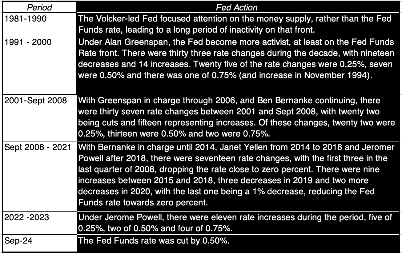
FFR is a range such as 5.00%-5.25%, so we usually use the effective FFR, which shrink to a figure.
The Figure below shows the move of effective FFR over time.
There are two periods that stand out.
- The first is the spike in the Fed Funds rate to more than 20% between 1979 and 1982, when Paul Volcker was Fed Chair, and represented his attempt to break the cycle of high inflation that had entrapped the US economy.
- The second was the drop in the Fed Funds rate to close to zero percent, first after the 2008 crisis and then again after the COVID shock in the first quarter of 2020. In fact, coming into 2022, the Fed had kept the Fed Funds rates at or near zero for most of the previous 14 years, making the surge in rates in 2022, in response to inflation, shock therapy for markets unused to a rate-raising Fed.

As noted that the Fed only set FFR, there are undoubtedly other interest rates you will encounter, but are not set by the Fed. Those other rates will fall into one of three buckets – (1) market-set interest rates, (2) rates indexed to market-set rates and (3) institutionally-set rates. None of these rates are set by the Federal Reserve, thus rendering the “Fed sets interest rates” as myth.
Myth 2. The Fed as Rate Leader
Although the Fed does not set rate directly, you may still believe that the Fed influences these rates with changes it makes to the Fed Funds rate.

The rates all seem to move in sync, though market-set rates move more than institution-set rates, which, in turn, are more volatile than the Fed Funds rate. The reason that this is a superficial test is because these rates all move contemporaneously, and there is nothing in this graph that supports the notion that it is the Fed that is leading the change. In fact, it is entirely possible, perhaps even plausible, that the Fed’s actions on the Fed Funds rate are in response to changes in market rates, rather than the other way around.
Some Statistics are provided by Professor Damodaran, as the Table below. To test whether changes in the Fed Funds rate are a precursor for shifts in market interest rates, a simple (perhaps even simplistic) test is provided. At the 249 quarters that compose the 1962- 2024 time period, each quarter was broken own into whether the effective Fed Funds rate increased, decreased or remained unchanged during the quarter. It seems undeniable that the “Fed as leader” hypothesis falls apart. In fact, in the quarters after the Fed Funds rate increases, US treasury rates (short and long term) are more likely to decrease than increase, and the median change in rates is negative. In contrast, in the periods after the Fed Fund decreases, treasury rates are more likely to increase than decrease, and post small median increases.
.jpeg)
Findings how that the Fed is more like an follower rather than a leader, when it comes to interest rate. What is the cause of the those interest rate then? How else can you explain why interest rates remained low for the last decades, other than the Fed?
The answer is recognizing that market-set rates ultimately are composed of two elements: (1) expected inflation rate and (2) expected real interest rate, reflecting real economic growth. In the graph below, which the professor have used multiple times in prior posts, he compute an intrinsic risk free rate by just adding inflation rate and real GDP growth each year:

The figure is like the Taylor Rule. Interest rates were low in the last decade primarily because inflation stayed low (the lowest inflation decade in a century) and real growth was anemic. Interest rates rose in 2022, because inflation made a come back, and the Fed scrambled to catch up to markets, and most interesting, interest are down this year, because inflation is down and real growth has dropped. As you can see, in September 2024, the intrinsic risk-free rate is still higher than the 10-year treasury bond rate, suggesting that there will be no precipitous drop in interest rates in the coming months.
Myth 3. The Fed as Signalman
There are two major macroeconomic dimensions on which the Fed collects data,
- (1) real economic growth (how robust it is, and whether there are changes happening), and
- inflation (how high it is and whether it too is changing).
The Fed’s major signaling device remains the changes in the Fed Funds rate, and it is worth pondering what the signal the Fed is sending when it raises or lowers the Fed Funds rate.
- On the inflation front, an increase or decrease in the Fed Funds rate can be viewed as a signal that the Fed sees inflationary pressures picking up, with an increase, or declining, with a decrease.
- On the economic growth front, an increase or decrease in the Fed Funds rate, can be viewed as a signal that the Fed sees the economy growing too fast, with an increase, or slowing down too much, with a decrease.
These signals get amplified with the size of the cut, with larger cuts representing bigger signals.
The 50bp cut on the 18th of Sep means the mix. If you are an optimist, you could take the action to mean that the Fed is finally convinced that inflation has been vanquished, and that lower inflation is here to stay. If you are a pessimist, the fact that it was a 50bp decrease, rather than the expected 25bp, can be construed as a sign that the Fed is seeing more worrying signs of an economic slowdown than have shown up in the public data on employment and growth. There is of course the cynical third perspective, which is that the Fed rate cut has little to do with inflation and real growth, and more to do with an election that is less than fifty days away.
In sum, signaling stories are alluring, and you will hear them in the coming days, from all sides of the spectrum (optimists, pessimists and cynics), but the truth lies in the middle, where this rate cut is good news, bad news and no news at the same time, albeit to different groups.
Myth 4. The Fed as Equity Market Whisperer
The Fed’s capacity to influence the interest rates that matter is limited, but you may still hold on to the belief that the Fed’s actions have consequences for stock returns. In fact, Wall Street has its share of investing mantras, including “Don’t fight the Fed”, where the implicit argument is that the direction of the stock market can be altered by Fed actions.
Based on the professor’s data, the S&P 500 did slightly better in quarters after the FFR decreased than when the rate increased, but reserved its best performance for quarters after those where there was no change in the FFR. Stock markets will be better served with fewer interviews and speeches from members of the FOMC and less political grandstanding (from senators, congresspeople and presidential candidates) on what the Federal Reserve should or should not do.
Myth 5. The Fed as Chanticleer
The Fed is like Chanticleer, with investors endowing it with powers to set interest rates and drive stock prices, since the Fed’s actions and market movements seem synchronized. As with Chanticleer, the truth is that the Fed is acting in response to changes in markets rather than driving those actions, and it is thus more follower than leader. That said, there is the very real possibility that the Fed may start to believe its own hype, and that hubristic central bankers may decide that they set rates and drive stock markets, rather than the other way around.
Conclusion
The delusion shall be broken. The Fed did not lead the market but follow the market. Analyse the instruction of Fed might miss the cause and effect. Should do analyse the following factors.
It has distracted us from talking about things that truly matter, which include growing government debt, inflation, growth and how globalisation may be feeding into risk, and allowed us to believe that central bankers have the power to rescue us from whatever mistakes we may be making.
The Fed Delusion has destroyed enough investing brain cells for those who holding on to the delusion cannot let go. Do not hear talking among this group about what the FOMC may or may not do at its next meeting (and the meeting after that), and what this may mean for markets, restarting the Fed Watch. The insanity of it all!
Reference
https://aswathdamodaran.blogspot.com/2024/09/fed-up-with-fed-talk-central-banks.html
Non-Violent Communication
by Marshall B. Rosenberg, PhD
The book is discussing about how to do compassionate communication, or Non-Volent Commutation. The abbreviation NVC.
1. Giving from the Heart
There raise two questions:
- What happens to disconnect us from our compassionate nature, leading us to behave violently and exploitative?
- What allows some people to stay connected to their compassionate nature under even the most trying circumstances?
NVC is a way of communicating that leads us to give from the heart.
We perceive relationships in a new light when we use NVC to hear our own deeper needs and those of others.
Generally, the book gives a NVC model with four components.
- (Part One) Observations. We observe what is actually happening in a situation.
The trick is to be able to articulate this observation without introducing any judgement or evaluation — to simply say what people are doing that we either like or don’t like.
-
(Part One) Feeling. We state how we feel when we observe this action, are we hurt scared, joyful, amused, irritated?
-
(Part One) Needs. We say what needs of ours are connected to the feelings we have identified.
-
(Part Two) Requests. The fourth component, requests, address what we are wanting from the other person that would enrich our lives or make life more wonderful for us.
We connect with people by first sensing what they are observing, feeling, and needing; then we discover what would enrich their lives by receiving the fourth piece — their request.
2. Communication That Blocks Compassion
- Moralistic Judgements.
One kind of life-alienating communication is the use of moralistic judgements that imply wrongness or badness on the part of people who don’t act in harmony with our values. (Don’t judge Good or Bad for others)
Don’t judge. Don’t do judgement, like “who is what”.
Analyses of others are actually expressions of our own needs and values.
It is important not to confuse value judgements and moralistic judgements. (We don’t do moralistic judgement, but can do value judgement).
- All of us make value judgements as to the qualities we value in life: for example, we might value honesty, freedom, or peace. Value judgements reflect our beliefs of how life can best to be served.
-
We make moralistic judgements of people and behaviours that fail to support our value judgement: for example, “Violence is bad. People who kill others are evil”
- Classifying and judging people promotes violence.
-
Make Comparisons.
Comparisons are a form of judgement. Making comparison blocks compassion.
-
Denial of Responsibility.
The use of the common expression have to, as in “There are some things you have to do, whether you like it or not”, illustrates how personal responsibility.
The phrase makes one feel, as in “You make me feel guilty”, is another example of how language facilitates denial of personal responsibility for our own feelings and thoughts.
-
Other Forms of Life-Alienating Communication.
Communicating our desires as demands is yet another form language that blocks compassion.
A demand explicitly or implicitly threatens listeners with blame or punishment if they fail to comply. It is a common form of communication in our culture, especially among those who hold positions of authority.
Thinking based on “Who deserves what” blocks compassionate communication.
Most of us grew up speaking a language that encourages us to label, compare, demand, and pronounce judgements rather than to be aware of what we are feeling and needing.
Four Components of NVC: Self-expression
3. Observing without Evaluating
The first component of NVC entails the separation of observation from evaluation.
- Observations are an important element in NVC, where we wish to clearly and honestly express how we are to another person. When we combine observation with evaluation, we decrease the likelihood that others will hear our intended message. Instead, they are apt to hear criticism and thus resist whatever we are saying .
-
NVC does not mandate that we remain completely objective and refrain from evaluating. It only requires that we maintain separation between our observations and our evaluations.
-
Don’t label even for positive words.
-
The highest form of human Intelligence.
The Indian philosopher J. Krishnamurti once remarked that observing without evaluating is the highest form of human intelligence.
-
Distinguishing Observations from Evaluations.
- The words always, never, ever, whenever, etc. express observations when used in the following ways
Whenever I have observed Jack on the phone, he as spoken for at least thirty minutes.
I cannot recall your ever writing to me.
- Sometimes such words are used as exaggerations, in which case observations and evaluations are being mixed:
You are always busy.
She is never there when she’s needed.
- When these words are used as exaggerations, they often provoke defensiveness rather than compassion.
Words like frequently and seldom can also contribute to confusing observation with evaluation.
4. Identifying and Expressing Feelings
The second component of NVC is to express how we are feeling.
- Feelings versus Non-feelings. The confusion, generated by the English language, is our use of the word feel without actually expressing a feeling.
Conversely, in the English language, it is not necessary to use the word feel at all when we are actually expressing a feeling: we can say, “I’m feeling irritated”, or simply “I’m irritated”.
So, distinguish between what we feel and what we think we are. Distinguish feelings from thoughts. For example,
- “I feel misunderstood“. The word “misunderstood” indicates the assessment of the other person’s level of understanding rather than any actual feeling.
- “I feel unimportant to the people with whom I work”. The word “unimportant” describes how I think others and evaluating me, rather than an actual feeling, which in this situation might be “I feel sad” or “I feel discouraged“.
- “I feel ignored”. The word “ignored” expresses how we interpret others, other than how we feel.
By developing a vocabulary of feelings that allows us to clearly and specifically name or identify our emotions, we can connect more easily with one another. Allowing ourselves to be vulnerable by expressing our feelings can help resolve conflicts.
5. Taking Responsibility for Our Feelings
The third component of NVC entails the acknowledgement of the root of our feelings.
NVC heightens our awareness that what others say and do may be the stimulus, but never the cause, of our feelings.
We see that our feelings result from how we choose to receive what others say and do, as well as from our particular needs and expectations in that moment. With this third component, we are led to accept responsibility for what we do to generate our own feelings.
- Four options for receiving negative messages:
- Blame ourselves
- Blame others
- Sense our own feelings and needs
- Sense others’ feelings and needs
We accept responsibility for our feelings, rather than blame other people, by acknowledging our own needs, desires, expectations, values, or thoughts.
-
The more we are able to connect our feelings to our own needs, the easier it is for others to respond compassionately.
Connect your feeling with your needs: “I feel … because I need …”
-
Distinguish between giving from the heart and being motivated by guilt.
The basic mechanism of motivating by guilt is to attribute the responsibility for one’s own feelings to others.
-
The needs at the Roots of Feelings.
Judgements of others are alienated expressions of our own unmet needs.
If someone says, “You never understand me,” they are really telling us that their need to be understood is not being fulfilled.
When we express our needs indirectly through the use of evaluations, interpretations, and images, others are likely to hear criticism. And when people hear anything that sounds like criticism, they tend to invest their energy in self-defense or counterattack.
So, what shall we do is to express our needs, and we would have a better chance of getting the needs met, as it would be easier for others to respond to us compassionately. And, if we don’t value our needs, others may not either.
-
From Emotional Slavery to Emotional Liberation.
- Stage 1: Emotional Slavery. W see ourselves responsible for others’ feelings.
We think we must constantly strive to keep everyone happy. Taking responsibility for the feelings of others can be very detrimental to intimate relationships.
- Stage 2: The obnoxious stage. We feel angry; we no longer want to be responsible for others’ feelings.
We become aware of the high costs of assuming responsibility for others’ feelings and trying to accommodate them at our own expense.
We tend toward obnoxious comments like, “Thant’s your problem! I’m not responsible for your feelings” when presented with another person’s pain.
- Stage 3: Emotional Liberation. We take responsibility for our intentions and actions.
We respond to the needs of others out of compassion, never out of fear, guilt, or shame.
6. Requesting That Which Would Enrich Life.
The fourth and final component of this process addresses what we would like to request of others in order to enrich life for us.
- Using positive Action Language.
We express what we are requesting rather than what we are not requesting. Do not request a “don’t”. Because “How do you do a don’t”? All I know is I feel won’t we I’m told to do a don’t.
-
Tell others what to do, while requesting. Don’t be vague.
In addition to using positive language, we also want to word our requests in the form of concrete actions that others can undertake and to avoid vague, abstract, or ambiguous phrasing.
Making requests in clear, positive, concrete action language reveals what we really want. Don’t make vague language, as vague language contributes to internal confusion.
For example, instead of saying “I want you to feel free to express yourself around me” , “I’d like you to tell me what I might do to make it easier for you to feel free to express yourselves around me”.
The first sentence do not actually tell the other to express what.
-
Making Requests Consciously.
When we simply express our feelings, it may not be clear to the listener what we want them to do.
We are often not conscious of what we are requesting. We talk to others or at them without knowing how to engage in a dialogue with them. We toss out words, using the presence of others as a wastebasket. In such situations, the listener, unable to discern a clear request in the speaker’s words, may experience the kind of distress.
Requests may sound like demands when unaccompanied by the speaker’s feelings and needs.
The clearer we are about what we want, the more likely it is that we’ll get it.
-
Asking for a Reflection.
To make sure the message we sent is the message that’s received, ask the listener to reflect it back.
Express appreciation when your listener tries to meet your request for a reflection.
When we first begin asking others to reflect back what they hear us say, it may feel awkward and strange because such requests are rarely made. When I emphasize the importance of our ability to ask for reflections, people often express reservations. They are worried about reactions like, “What do you think I am — deaf?” or, “Quit playing your psychological games.” To prevent such responses, we can explain to people ahead of time why we may sometimes ask them to reflect back our words. We make clear that we’re not testing their listening skills, but checking out whether we’ve expressed ourselves clearly.
-
Requesting Honesty
After we express ourselves vulnerably, we often want to know:
- What the listener is feeling.
We’d like to know the feelings that are stimulated by what we said, and the reasons for those feelings. For example, by asking. “I would like you to tell me how you fell about what I just said, and your reasons for feeling as you do”.
-
What the listener is thinking.
Specify which thoughts we’d like them to share. For example, we might say, “I’d like you to tell me if you predict that my proposal would be successful, and if not, what you believe would prevent its success.” rather than simply saying, “I’d like you to tell me what you think about what I’ve said.” When we don’t specify which thoughts we would like to receive, the other person may respond at great length which thoughts that aren’t the ones we are seeking.
-
Whether the listener would be willing to take a particular action.
For example, by asking, “I would like you to tell me if you would be willing to postpone our meeting for one week.”
- What the listener is feeling.
-
Requests versus Demands
Requests are good, while Demands are bad.
Our requests are received as demands when others believe they will be blamed or punished if they do not comply. When people hear a demand, they see only two options: submission or rebellion. Either way, the person requesting is perceived as coercive, and the listener’s capacity to respond compassionately to the request is diminished.
The more we have in the past blamed, punished, or “laid guilt trips” on others when they haven’t responded to our requests, the higher the likelihood that our requests will now be heard as demands. We also pay for others’ use of such tactics. To the degree that people in our lives have been blamed, punished, or urged to feel guilty for not doing what others have requested, the more likely they are to carry this baggage to every subsequent relationship and hear a demand in any request.
It’s a demand if the speaker then lays a guilt trip.
We can help others trust that we are requesting, not demanding by indicating that we would only want them to comply if they can do so willingly. Thus we might ask, “Would you be willing to see the table?” rather than “I would like you to set the table.” However, the most powerful way to communicate that we are making the most powerful way to communicate that we are making a genuine request is to empathise with people when they don’t agree to the request.
-
Defining our objective when making requests.
Expressing genuine requests also requires an awareness of our objective. If our objective is only to change people and their behaviour or to get our way, then NVC is not an appropriate tool.
The objective of NVC is not to change people and their behaviour in order to get our way; it is to establish relationships based on honesty and empathy that will eventually fulfill everyone’s needs.
Our objective is a relationship based on honesty and empathy.
Four Components of NVC: Apply to others
7. Receiving Emphatically
We refer the communication process that contains observing, feeling, needing, and requesting, as receiving emphatically
- Empathy is not just hearing.
The hearing that is only in the ears is one thing. The hearing of the understanding is another. But the hearing of the spirit is not limited to any one faculty, to the ear, or to the mind.
Bad: give advice or reassurance and to explain our own position or feeling.
Good: The true empathy requires us to focus full attention on the other person’s message. We give to others the time and space they need to express themselves fully and to feel understood.
Intellectual understanding blocks empathy. Questions such as, “when did this begin?” constituted the most frequent response; they give the appearance that the professional is obtaining the information necessary to diagnose and then treat the problem. In fact, such intellectual understanding of a problem blocks the kind of presence that empathy requires.
The key ingredient of empathy is presence: we are wholly present with the other party and what they are experiencing.
-
Listening for feelings and needs.
No matter what words people use to express themselves, we listen for their (1)observations, (2)feelings, (3)needs, and (4)requests.
To listen to what people are needing rather than what they are thinking. People would be less threatening if you hear what they’re needing rather than what they’re thinking about you. Instead of hearing that he’s unhappy because he thinks you don’t listen, focus on what he’s needing by saying, “Are you unhappy because you are needing…”
-
Paraphrasing.
After we focus our attention and hear what others are observing feeling, and needing and what they are requesting to enrich the lives, we may wish to reflect back by paraphrasing what we understood.
Advantages:
- If we have accurately received the other party’s message, our paraphrasing will confirm this for them. If, on the other hand, the paraphrase is incorrect, we give the speaker an opportunity to correct us.
- Paraphrasing offer people time to reflect on what they’ve said and an opportunity to delve deeper into themselves.
How to Do: Paraphrasing take the form of questions that reveal our understanding while eliciting any necessary corrections from the speaker.
Questions may focus on these components:
- What others are observing: “Are you reacting to how many evenings I was gone last week?”
- how others are feeling and the needs generating their feelings: “Are you feeling hurt because you would have liked more appreciation of your efforts than you received?”
- what others are requesting: “Are you wanting me to tell you my reasons for saying what I did?”
- Do the questions like above, not the followings, as the above invite others’ corrections.
1.“What did I do that you are referring to?” 2. “How are you feeling?” “Why are you feeling that way?” 3. “What are you wanting me to do about it?”
This second set of questions asks for information without first sensing the speaker’s reality.
When asking for information, first express our own feelings and needs. Because schoolteacher types questions are too straight forward. People would prefer questions that reveals the feelings and needs within ourselves, and show feelings make people feel safer.
i.e. Instead of asking “What did I do?”, we might say, “I’m frustrated because I’d like to be clearer about what you are referring to. Would you be willing to tell me what I’ve done that leads you to see me in this way”
-
Sustaining Empathy.
I recommend allowing others the opportunity to fully express themselves before turning our attention to solutions or requests for relief. When we proceed too quickly to what people might be requesting, we may not convey our genuine interest in their feelings and needs; instead, they may get the impression that we’re in a hurry to either be free of them or to fix their problem.
By maintaining our attention on what’s going on within others, we offer them a chance to fully explore and express their interior selves.
We know a speaker has received adequate empathy when (1) we sense a release of tension, or (2) the flow of words comes to a halt.
8. The Power of Empathy
Empathy allows us “to re-perceive [our] world in a new way and to go on.”
- Empathy and the Ability to Be Vulnerable
Because we are called to reveal our deepest feelings and needs, we may sometimes find it challenging to express ourselves in NVC.
Self-expression becomes easier, however, after we empathise with others, because we will then have touched their humanness and realized the common qualities we share. The more we connect with the feelings and needs behind their words, the less frightening it is to open up to other people.
-
Empathy for Silence
Empathise with silence by listening for the feelings and needs behind it.
9. Connecting Compassionately with Ourselves
-
Translating Self-Judgements and Inner Demands.
Self-judgements, like all judgements, are tragic expressions of unmet needs.
A basic premise of NVC is that whenever we imply that someone is wrong or bad, what we are really saying is that he or she is not acting in harmony with our needs. If the person we are judging happens to be ourselves, what we are saying is, “I myself am not behaving in harmony with my own needs.” I am convinced that if we learn to evaluate ourselves in terms of whether and how well our needs are being fulfilled, we are much more likely to learn from the evaluation.
-
NVC Mourning
Mourning in NVC is the process of fully connecting with the unmet needs and the feelings that are generated when we have been less than perfect. It is an experience of regret, but regret that helps us learn from what we have done without blaming or hating ourselves.
We can train ourselves to recognise judgemental self-talk and to immediately focus our attention on the underlying needs.
-
Self-Forgiveness.
When were listen emphatically to ourselves, we will be able to hear the underlying need. Self-forgiveness occurs the moment this emphatic connection is made.
NVC Self-Forgiveness: connecting with the need we were trying to meet when we took the action that we now regret.
The process of mourning and self-forgiveness frees us in the direction of learning and growing.
-
Don’t Do Anything That Isn’t Play
Do things that are playful. We want to take action out of the desire to contribute to life rather than out of fear, guilt, shame, or obligation. Here are some possible ways:
- Translating “Have to” to “Choose to”
With every choice you make, be conscious of what need it serves.
-
Cultivating Awareness of the Energy Behind Our Actions.
Consider the statement “I choose to … because I want …”. Be careful with the important values behind the choices you have made.
- For Money
- For Approval
- To Escape Punishment
- To Avoid Shame
- To Avoid Guilt
- To Satisfy A Sense of Duty
- Translating “Have to” to “Choose to”
10. Expressing Anger Fully
-
The Core of Anger
All angers are as a result of life-alienating, violence-provoking thinking. At the core of all anger is the need that is not being fulfilled. Thus anger can be valuable if we use it as an alarm clock to wake us up — to realise we have a need that isn’t being met and that we are thinking in a way that makes it unlikely to be met.
-
Four Steps to Expressing Anger.
- Stop and do nothing except to breathe. We refrain from making any move to blame or punish the other person. We simply stay quiet.
- Identify the thoughts that are making us angers
- Connect with our needs. We know that all judgements are tragic expressions of unmet needs, so we take the next step and connect to the needs behind those thoughts.
- Express our feelings and unmet needs. We open our mouth and speak the anger — but the anger has been transformed into needs and need-connected feelings.
- Offering Empathy First.
Another step needs to take place before we can expect the other party to connect with what is going on in us. Offer Empathy First.
- The more we hear them, the more they’ll hear us.
-
Stay conscious of the violent thoughts that arise in our minds, without judging them.
-
When we hear another person’s feelings and needs, we recognise our common humanity.
11. Conflict Resolution and Mediation
This topics is regarding addressing how to apply NVC in resolving conflicts.
- Human Connection.
Create connection between the people who are in conflict is the most important thing.
-
Steps.
- Express our own needs.
- Seek the real needs of the other person. Seek the need behind their words, the need underneath what they are saying.
- Verify that we both accurately recognise the other person’s needs.
- Provide as much empathy, mutually hearing each other’s needs accurately.
- Propose strategies for resolving the conflict.
P.S. Avoid the use of language that implies wrongness. Listen to each other with utmost care.
-
On Needs, Strategies, and Analysis.
Fundamentally, needs are the resources life requires to sustain itself. Consider difference between a person’s needs and his or her strategy for fulfilling them, and make strategies.
Sensing others’ needs, no matter what they’re saying.
Using present and positive action language to resolve conflict.
The use of NVC to resolve conflict differs from traditional mediation methods; instead of deliberating over issues, strategies, and means of compromise, we concentrate foremost on identifying the needs of both parties, and only then seek strategies to fulfill those needs.
We start by forging a human connection between the parties in conflict. Then we ensure that both parties have the opportunity to fully express their needs, that they carefully listen to the other person’s needs, and that once the needs have been heard, they clearly express doable action steps to meet those needs. We avoid judging or analysing the conflict and instead remain focused on needs.
When one party is in too much pain to hear the needs of the other, we extend empathy, taking as long as necessary to ensure that the person knows their pain is heard. We do not hear “no” as a rejection but rather as an expression of the need that is keeping the person from saying “yes”. Only after all needs have been mutually heard, do we progress to the solution stage: making doable request using positive, action language.
When we assume the role of mediating a conflict between two other parties, the same principles apply. In addition, we keep careful track of progress, extend empathy where needed, keep the conversation focused on the present, moving it forward, and interrupting where necessary to return to the process.
With these tools and understanding, we can practice and help others resolve even long-standing conflicts to their mutual satisfaction.
12. The Protective Use of Force
In situations where there is no opportunity for communication, such as in instances of imminent danger, we may need to resort to the protective use of force. The intention behind the protective use of force is to prevent injury or injustice, never to punish or to cause individuals to suffer, repent, or change. The punitive use of force tends to generate hostility and to reinforce resistance to the very behaviour we are seeking. Punishment damages goodwill and self-esteem, and shifts our attention from the intrinsic value of an action to external consequences. Blaming and punishing fail to contribute to the motivations we would like to inspire in others.
13. Liberating Ourselves and Counselling Others.
Apply the NVC to ourselves, in order to enhances inner communication by helping us translate negative internal messages into feelings and needs. Our ability to distinguish our own feelings and needs and to empathise with them can free us from depression.
14. Expressing Appreciation in Nonviolent Communication
Research shows that if a manager compliments employees, they work harder. And the same goes for schools: if teachers praise students, they study harder. The author have reviewed this research, and find that recipients of such praise do work harder, but only initially. Once they sense the manipulation behind the appreciation, their productivity drops.
When we use NVC to express appreciation, it is purely to celebrate, not to get something in return.
- The Three Components of Appreciation
- the actions that have contributed to our well-being;
- the particular needs of ours that have been fulfilled;
- the pleasureful feelings engendered by the fulfilment of those needs
The sequence of these ingredients may vary; sometimes all three can be conveyed by a smile or a simple “Thank you.” However, if we want to ensure that our appreciation has been fully received, it is valuable to develop the eloquence to express all three components verbally.
-
We shall overcome the reluctance to express appreciation.
-
When we receive appreciation expressed in this way, we can do so without any feeling of superiority or false humility—instead we can celebrate along with the person who is offering the appreciation.
Atomic Habits
by James Clear
The book tells how to cultivate habits.
The author states the following. As changes that seem small and unimportant at first will compound into remarkable results if you’re willing to stick with them for years. We all deal with setbacks but in the long run, the quality of our lives often depends on the quality of our habits. With the same habits, you’ll end up with the same results. But with better habits, anything is possible.
The backbone of this book is the author’s four-step model of habits–cue, craving, response, and reward–and the four laws of behaviour change that evolve out of these steps.
The Fundamentals – Why Tiny Changes Make a Big Difference
1 The Surprising Power of Atomic Habits
- The relentless commitment to a strategy make a Cycling Coach outstanding than others (referred as “the aggregation of marginal gains”, which was the philosophy of searching for a tiny margin of improvement in everything you do). The whole principle of this coach is if you broke down everything you could think of that goes into riding a bike, and then improve it by 1 percent, you will get a significant increase when you put them all together.
-
As these and hundreds of other small improvements accumulated, the results came faster than anyone could have imagined.
But when we repeat 1 percent errors, day after day, by replicating poor decisions, duplicating tiny mistakes, and rationalising little excuses, our small choices compound into toxic results.
Making a choice that is 1 percent better or 1 percent worse seems insignificant in the moment, but over the span of moments that make up a lifetime these choice determine the difference between who you are and who you could be. Success is the product of daily habits–not once-in-a-lifetime transformations.
-
Time magnifies the margin between success and failure. It will multiply whatever you feed it. Good habits make time your ally. Bad habits make time you enemy.
-
Forget about goals, focus on systems instead.
What’s the difference between systems and goals? Goals are about the results you want to achieve. Systems are about the processes that lead to those results.
Goals are good for setting a direction, but systems are best for making progress.
A handful of problems arise when you spend too much time thinking about your goals and not enough time designing your systems.
- Problem #1: Winers and losers have the same goals.
Goal setting suffers from a serious case of survivorship bias. People who end up with winning–the survivors–and mistakenly assume that ambitious goals led to their success while overlooking all of the people who had the same objective but didn’t succeed.
Nobody has the goal of losing, but only winners prove with the goal.
- Problem #2: Achieving a goal is only a momentary change.
When you solve problems at the results level, you only solve them temporarily. In order to improve for good, you need to solve problems at the systems level. Fix the inputs and outs will will fix themselves.
- Problem #3: Goals restrict your happiness. Goals create an “either-or” conflict: either you achieve your goal and are successful or you fail and you are a disappointment. Do not link goals with happiness, instead link with the process. When you fall in love with the process rather than the product, you don’t have to wait to give yourself permission to be happy. You can be satisfied anytime your system is running.
-
Problem #4 Goals are at odds with long-term progress. A goal-oriented mindset can create a “yo-yo” effect. Many runners work hard for months, but as soon as they cross the finish line, they stop training. The purpose of setting goals is to win the game. The purpose of building systems is to continue playing the game. Have a long-term thinking, and do not be goal-oriented.
-
If you’re having trouble changing your habits, the problem isn’t you. The problem is your system. Focusing on the overall system rather than a single goal, is one of the core themes of this book.
The atomic habit refers to a tiny change, a marginal gain, a 1 percent improvement. Atomic habits are the building blocks of remarkable results.
2 How Your Habits Shape Your Identity (and Vice Versa)
Few things can have a more powerful impact on your life than improving your daily habits. However, once your habits are established, they seem to stick around forever–especially the unwanted ones.
- There are three layers of behaviour changes:
- The first layer is changing your outcomes/results.
-
The second layer is changing your process, changing the habits and systems
-
The third and deepest layer is changing your identity, changing the beliefs, the worldview, the self-image, etc.
-
Outcomes are about what you get. Processes are about what you do. Identity is about what you believe.
-
Many people begin the process of changing their habits by focusing on what they want to achieve. This leads us to outcome-based habits. The alternative is to build identity-based habits. With this approach, we start by focusing on who we wish to become.
-
The ultimate form of intrinsic motivation is when a habit becomes part of your identity. True behaviour change is identity change. You might start a habit because of motivation, but the only reason you’ll stick with one is that it becomes part of your identity. i.e.
- The goal is not to read a book, the goal is to become a reader/
-
The goal is not to run a marathon, the goal is to become a runner.
-
The goal is not to learn an instrument, the goal is to become a musician.
-
The Shaping Identity is a double-edged sword. The deeply a thought or action is tied to your identity, the more difficult it is to change it.
-
A two-step process to changing your identity.
- Decide the type of person you want to be.
- Prove it to yourself with small wins.
- The more you repeat a behaviour, the more you reinforce the identity associated with the behaviour.
-
The more evidence you have for a belief, the more strongly you will believe it.
The process of building habits is actually the process of becoming yourself.
- Small habits can make a meaning full difference by proving evidence of a small identity.
- Use the feedback loops. Once you have a handle on the type of person you want to be, you can begin taking small steps to reinforce your desired identity. Your habits shape your identity, and your identity shapes your habits.
-
To cultivate a habit. The first step is not what or how, but who.
3. How to Build Better Habits in 4 Simple Steps
Scholar, Thorndike, described the learning process, “Behaviours followed by satisfying consequences tend to be repeated and those that produce unpleasant consequences are less likely to be repeated”
- Why the Brain builds habits?
Whenever you encounter a new situation in life, the brain has to make a decision. Neurological activity in the brain is high during the period.
As habits are created, the level of activity in the brain decreases. When a similar situation arises in the future, you know exactly what to look for. There is no longer a need to let the brain think and make decision and analyse every angle of a situation.
In short, habits are mental shortcuts learned from experience.
Habits reduce cognitive load and free up mental capacity, so you can allocate your attention to other tasks.
Habits do not restrict freedom. They create it. In fact, the people who don’t have their habits handled are often the ones with the least amount of freedom, because the brain is always overloaded.
When you have habits dialed in and the basics of life are handled and done, your mind is free to focus on new challenges and master the next set of problems.
-
The process of building a habit.
Four simple steps: cue, craving, response, and reward.
- Cue triggers your brain to initiate a behaviour.
- Cravings are the motivational force behind every habit.
- Response is the actual habit you perform, which can take the form of a thought or an action.
- Rewards are delivered by Response. There are two purposes of reward. (1) Reward satisfy your craving. (2) reward teaches us which actions are worth remembering in the future.
- The author would illustrate those four steps in details later.
- The four steps make a loop, and reinforce the process. The cue triggers a craving, which motivates a response, which provides a reward, which satisfies the craving and, ultimately, becomes associated with the cue.
- The four laws of behaviour change.
- The 1st Law (Cue) <– Make it obvious.
- The 2nd Law (Craving) <– Make it attractive.
- The 3rd Law (Response) <– Make it easy.
- The 4th Law (Reward) <– Make it satisfying.
- For bad habits, do the reveres. Make the cue invisible, make craving unattractive, make response difficult, and make reward unsatisfying.
The 1st Law: Make it Obvious
4. The Man who didn’t Look Right
- With enough practice, your brain will pick up on the cues that predict certain outcomes without consciously thinking about it.
- Once the habits become automatic, we stop paying attention to what we are doing.
- The process of behaviour change always starts with awareness. You need to be aware of your habits before you can change them.
5. The Best Way to Start a New Habit
- The 1st law of Behaviour Change is make it obvious.
-
Two most common cues are time and location. Create the Implementation Intention, which is a plan you make beforehand about when and where to act. That is, how you intend to implement a particular habit. Like “When situation X arises, I will perform response Y”. Or, I will [BEHAVIOUR] at [TIME] in [ LOCATION].
-
Many human behaviours follow a chain reaction cycle. You decide what to do next based on what you have just finished doing (Bayesian). No behaviours happen in isolation. Each action becomes a cue that triggers the next behaviour.
-
Habit Stacking. Inspired by the above, when it comes to building new habits, you can use the connectedness of behaviour to your advantage. One of the best ways to build a new habit is to identify a current habit you already do each day, and then stack your new behaviour on the top. In a word, linking one behaviour with the other.
-
Tie your desired behaviour into something you already do each day. Once you have mastered this basic structure, you can begin to create larger stacks by chaining small habits together. The habit stacking allows you to create a set of simple rules that guide your future behaviour.
In short, After I [CURRENT HABIT], I will [NEW HABIT].
6. Motivation is Overrated, Environment Often Matters More
People Often choose products not because of what they are, but because of where they are. Environment is the invisible hand that shapes human behaviour.
In this way, the most common form of change is not internal, but external: we are changed by the world around us. Every habit is context dependent.
By psychologist Kurt Lewin (1936): Behaviour is a function of Person in their Environment, B=f(P,E).
- In humans, perception is directed by the sensory nervous system. We perceive the world through sight, sound, smell, touch, and taste. And other ways of sensing stimuli, some are conscious, but many are non-conscious. Receptors in your body pick up on a wide range if internal stimuli. One of the most powerful human sensory abilities is vision. A small change in what you see can lead to a big shift in what you do.
-
The environments where we live and work often make it easy not to do certain actions because there is no obvious cue to trigger the behaviour. What we do is to make it visually obvious. We shall change the environment.
-
Environment design is powerful not only because it influences how we engage with the world but also because we rarely do it.
-
Create the the Context of Cue.
Over time, your habits become associated not with a single trigger but with the entire context surrounding the behaviour.
The behaviour is not defined by the objects in the environment but by our relationship to them. Thank in terms of how you interact with the spaces around you.
The power of context reveals an important strategy: habits can be easier to change in a new environment.
Whenever possible, avoiding mixing the context of one habit with another. The inspiration is to split the Space to Work, and the Space to Study and Live.
If your space is limited, divide your room into activity zones: a chair for reading, a desk for writing, a table for eating, etc.
7. The Secret to Self-Control
When scientists analyse people who appear to have tremendous self-control, it turns out those individuals aren’t all the different from those who are struggling. Instead, “disciplined” people are better at structuring their lives in a way that does not require heroic willpower and self-control. In other words, they spend less time in tempting situations.
- Bad habits are auto-catalytic: the process feeds itself.
One of the most practical ways to eliminate a bad habit is to reduce exposure to the cue that causes it.
The practice is an inversion of the 1st Law of Behaviour Change. Rather than make it obvious, you can make it invisible (for the bad habit).
The 2nd Law: Make it Attractive
8. How to Make a Habit Irresistible
Scientists refer to exaggerated cues as supernormal stimuli, which is a heightened version of reality and elicits a stronger response than usual. They exaggerate features that are naturally attractive to us, and our instincts go wild as a result, driving us into excessive shopping habits, social media habits, porn habits, eating habits, and many others. Hereafter are some biological response.
- The Dopamine-Driven Feedback Loop
Dopamine is not the only chemical that influences your habits, but it is the one that provide a window into the biological underpinnings of desire, craving, and motivation that are behind every habits.
For years, scientists assumed dopamine was all about pleasure, but now we know it plays a central role in many neurological processes, including motivation, learning and memory, punishment and aversion, and voluntary movement.
When it comes to habits, the key takeaway is this: dopamine is released not only when you experience pleasure, but also when you anticipate it.
The more attractive an opportunity is, the more likely it is to become habit-forming.
-
Use the Temptation Bundling to make your habits more attractive.
Temptation bundling works by linking an action you want to do with an action you need to do.
9. The Role of Family and Friends in Shaping Your Habits
-
The Seductive Pull of Social Norms: Humans are herd animals. We want to fit in, to bond with others, and to earn the respect and approval of our peers.
Those who collaborated and bonded with others enjoyed increased safety, mating opportunities, and access to resources.
We imitate the habits of three groups in particulars:
- The close.
As a general rule, the closer we are to someone, the more likely we are to imitate some of their habits. Our friends and family provide a sort of invisible peer pressure that pulls us in their direction. We soak up the qualities and practices of those around us.
One of the most effective things you can do to build better habits is to join a culture where your desired behaviour is the normal behaviour. Join a culture where (1) your desired behaviour is the normal behaviour and (2) you already have something in common with the group.
Conversely, peer pressure is bad only if you’re surrounded by bad influences.
-
The many.
The normal behaviour of the tribe often overpowers the desired behaviour of the individual.
Humans are similar. There is tremendous internal pressure to comply with the norms of the group. The reward of being accepted is often greater than the reward of winning an argument, looking smart, or finding truth.
-
The powerful.
We try to copy the behaviour of successful people because we desire success ourselves.
High-status people enjoy the approval, respect, and praise of others. And the means if a behaviour can get us approval, respect, and praise, we find it attractive.
- The close.
10. How to Find and Fix the Causes of Your Bad Habits
-
Habits are all about associations. There associations determine whether we predict a habit to be worth repeating or not. The brain is continually absorbing information and noticing cues in the environment. Every time you perceive a cue, your brain runs a simulation and makes a prediction about what to do in the next moment.
The cause of your habits is actually the prediction that precedes them.
There predictions lead to feelings, which is how we typically describe a craving — a feeling, a desire, an urge. Feelings and emotions transform the cues we perceive and the predictions we make into a signal that we can apply.
To summaries, the specific cravings you feel and habits you perform are really an attempt to address your fundamental underlying motives. Whenever a habit successfully addresses a motive, you develop a craving to do it again.
Habits are attractive when we associate them with positive feelings, and we can use this insight to our advantage rather than to our detriment.
-
Reprogram Your Brain to Enjoy Hard Habits.
Changing just one word: You don’t “have” to You “get” to.
Transition from seeing there behaviours as burdens and turn them into opportunities.
Re-framing your habits to highlight their benefits rather than their drawbacks is a fast and light wight way to reprogram your mind and make a habit seem more attractive.
If you want to take it a step further, you can crate a motivation ritual. You simply practice associating your habits with something you enjoy, then you can use that cue whenever you need a bit of motivation.
Three deep breaths. Smile. Ped the dog. Repeat.
Eventually, you’ll begin to associate this breathe-and-smile routine with being in a good mood. It becomes a cue that means feeling happy.
The key to finding and fixing the causes of your bad habits is to re-frame the associations you have about them. It’s not easy, but if you can reprogram your predictions, you can transform a hard habit into an attractive one.
The 3rd Law: Make it Easy
11. Walk Slowly, but Never Backward
When you’re in motion, you’re planning and strategising and learning.
Action is the type of behaviour that will deliver an outcome.
If you want to master a habit, the key is to start with repetition, not perfection. You don’t need to map out every feature of a new habit. You just need to practice it.
Get start, try and protect, get exploration, not prepare for perfection.
- How long does it actually take to form a new habit?
The more you repeat an activity, the more the structure of your brain changes to become efficient at that activity. Neuroscientists call this long-term potentiating, which refers to the strengthening of connections between neurons in the brain based on recent patterns of activity. With each repetition cell-to-cell signaling improves and the neural connections tighten.
-
Repetition is a form of change
An English philosopher George H Lewes noted, “In learning to speak a new language, to play on a musical instrument, or to perform unaccustomed movements, great difficulty is felt, because the channels through which each sensation has to pass have not become established; but no sooner has frequent repetition cut a pathway, than this difficulty vanishes; the actions become so automatic that they can be performed while the mind is otherwise engaged.”
-
All habits follow a similar trajectory from effortful practice to automatic behavior, a process known as automaticity. Automaticity is the ability to perform a behaviour without thinking about each step, which occurs when the non-conscious mind takes over.
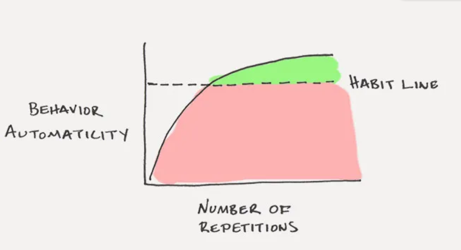
In practice, it doesn’t really matter how long it takes for a habit to become automatic. What matters is that you take the actions you need to take to make progress. Whether an action is fully automatic is of less importance.
12. The Law of Least Effort
- Habits like scrolling on our phones, checking email, and watching television steal so much of our time because they can be performed almost without effort. They are remarkable convenient.
-
You don’t actually want the habit itself. What you really want is the outcome the habit delivers. The greater the obstacle — that is, the more difficult the habit — the more friction there is between you and your desired end state. This is why it is crucial to make your habits so easy that you’ll do them even when you don’t feel like it. If you can make your good habits more convenient, you’ll be more likely to follow through on them.
-
The less friction you face, the easier it is for your stronger self to emerge. The idea behind make is easy is not only do easy things. The idea is to make it as easy as possible in the moment to do things that payoff in the long run.
- Reduce the friction associated with good behaviours. When friction is low, habits are easy. Increase the griction associated with bad behaviours. When friction is high, habits are difficult.
- Prime your environment to make future actions easier.
13. How to Stoop Procrastinating by Using the Two-Minute Rule
-
The Two-Minute Rule. Even when you know you should start small, it’s easy to start too big. When you dream about making a change, excitement inevitably takes over and you end up trying to do too much too soon. The most effective way I know to counteract this tendency is to use the Two-Minute Rule, which states, “When you start a new habit, it should take less than two minutes to do”.
A new habit should not feel like a challenge. The actions that follow can be challenging, but the first two minutes should be easy. What you want is a “gateway habit” that naturally leads you down a more productive path.
-
For Example: You can usually figure out gateway habits that will lead to your desired outcome by mapping out your goals on a scale from “very easy” to “very hard”. For instance, running a marathon is very hard. Running a 5K is hard. Walking ten thousand steps is moderately difficult. Walking ten minutes is easy. And putting on your running shoes is very easy. Your goal might be to run a marathon, but your gateway habit is to put on your running shoes. That’s how you follow the Two-Minute Rule.
-
focusing on just the first two minutes and mastering that stage before moving on the next level. Eventually, you’ll end up with the habit you had originally hoped to build while still keeping your focus where it should be: on the first two minutes of the behaviour.
14. How to Make Good Habits Inevitable and Bad Habits Impossible
-
Usecommitment device, a choice you make in the present that controls your actions in the future.
-
The best way to break a bad habit is to make it impractical to do. Increase the friction until you don’t even have the option to act.
- Onetime choices — like buying a better mattress or enrolling in an automatic savings plan — are single actions that automate your future habits and deliver increasing returns over time.
The 4th Law: Make It Satisfying
15. The Cardinal Rule of Behaviour Change
We are more likely to repeat a behaviour when the experience is satisfying. Conversely, if an experience is not satisfying, we have little reason to repeat it.
- The first three laws of behaviour change — make it obvious, make it attractive, and make it easy — increase the odds that a behaviour will be performed this time. The fourth law of behaviour change — make it satisfying — increases the odds that a behaviour will be repeated next time. It completes the habit loop.
-
However, there is a trick. Your human nature live in what scientists call an immediate-return environment because your actions instantly deliver clear and immediate outcomes. Yet, you, per se, live in what scientists call a delayed-return environment because you can work for years before your actions deliver the intended payoff.
The world has changed much in recent years, but human nature has changed little. The world becomes more Rewards-Delayed, but human nature needs Rewards-Immediate.
The brain’s tendency to prioritise the present moment means you can’t rely on good intentions.
-
Every habit produces multiple outcomes across time. Unfortunately, these outcomes are often misaligned. With our bad habits, the immediate outcome usually feels good, but the ultimate outcome feels bad. With good habits, it is the reverse: the immediate outcome is enjoyable, but the ultimate outcome feels good.
In other words, the costs of your good habits are in the present. The costs of your bad habits are in the future.
-
Cardinal Rule of Behaviour Change: What is immediately rewarded is repeated. What is immediately punished is avoided.
-
You need to work with the grain of human nature, not against it. The best way to do this is to add a little bit of immediate pleasure to the habits that pay off in the long-run and a little bit of immediate pain to ones that don’t/ Cultivate habits by artificially rewards yourself to the human nature.
To select short-term rewards that reinforce your identity rather than ones that conflict with it.
-
In summary, a habit needs to be enjoyable for it to last.
16. How to Stick with Good Habits Every Day
Making progress is satisfying, and visual measures — like moving paper clips or hairpins or marbles — provide clear evidence of your progress. As a result, they reinforce your behaviour and add a little bit of immediate satisfaction to any activity.
- Use habit track. Habit tracking (1) creates a visual cue that can remind you to act, (2) is inherently motivating because you see the progress you are making and don’t want to lose it, and (3) feels satisfying whenever you record another successful instance of your habit.
- What can we do to make tracking easier? First, whenever possible, measurement should be automated. Second, manual tracking should be limited to your most important habits. Finally, record each measurement immediately after the habit occurs.
- How to recover quickly when your habits were interrupted? Never miss twice. Try to not break the Chain.
17. How an Accountability Partner Can Change Everything
- The more immediate the pain, the less likely the behaviour. If you want to prevent bad habits and eliminate unhealthy behaviours, then adding an instant cost to the action is a great way to reduce their odds.
-
An accountability partner can create an immediate cost to inaction. We care deeply about what others think of us, and we do not want others to have a lesser opinion of us.
-
A habit contract can be used to add a social cost to any behaviour. It makers the costs of violating your promises public and painful.
Just as governments use laws to hold citizens accountable, you can create a habit contract to hold yourself accountable.
Advanced Tactics: How to Go from Being Merely Good to Being Truly Great
18. The Truth About Talent (When Genes Matter and When They Don’t)
The secret to maximising the odds of success is to choose the right field of competition. In short: Genes don’t determine your destiny. They determine your areas of opportunity.
- How your personality influences your habits:
- Openness to experience
- Conscientiousness
- Extroversion
- Agreeableness
- Neuroticism
Our habits are not solely determined by our personalities, but there is no doubt that our genes nudge us in a certain direction.
The Takeaway is that you should build habits that work for your personality. You don’t have to build the habits everyone tells you to build. Choose the habit that best suits you, not the one that is most popular.
-
How to find a game where the odds are in your favour:
- In the beginning of a new activity, there should be a period of exploration. The goal is to try out many possibilities, research a broad range of ideas, and cast a wide net.
- After this initial period of exploration, shift your focus to the best solution you’ve found — but keep experimenting occasionally.
- In the long-run it is probably most effective to work on the strategy that seems to deliver the best results about 80 to 90 percent of the time and keep exploring with the remaining 10 to 20 percent.
When you can’t win by being better, you can win by being different. By combining your skills, you reduce the level of competition, which makes it easier to stand out.
-
How to getthe most out of your genes:
The genes do not eliminate the need for hard work. They clarify it. They tell us what to work hard on. Once we realise our strengths, we know where to spend our time and energy.
In summary , one of the best ways to ensure your habits remain satisfying over the long-run is to pick behaviours that align with your personality and skills. Work hard on the things that come easy.
19. The Goldilocks Rule: How to Stay Motivated in Life and Work
The way to maintain motivation and achieve peak levels of desire is to work on tasks of “just manageable difficulty”.
The human brain loves a challenge, but only if it is within an optimal zone of difficulty.
- The Goldilocks Rule states that humans experience peak motivation when working on tasks that are right on the edge of their current abilities. Not too hard. Not too easy. Just right.
When you’re starting a new habit, it’s important to keep the behaviour as easy as possible so you can stick with it even when conditions aren’t perfect.
Once the habit has been established, it is important to continue to advance in small ways.
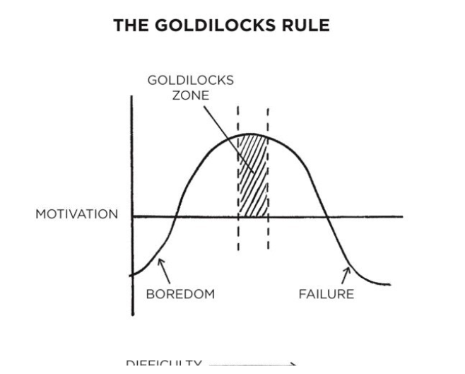
-
How to stay focused when you get bored working on your goals
The greatest threat to success is not failure but boredom.
Variable rewards won’t create a craving, but they are a powerful way to amplify the cravings we already experience because they reduce boredom.
-
Professionals stick to the schedule; amateurs let life get in the way. Professionals know what is important to them and work toward it with purpose; amateurs get pulled off course by the urgencies of life.
The only way to become excellent is to be endless fascinated by doing the same thing over and over. You have to fall in love with boredom
20. The Downside of Creating Good Habits
Habits are necessary, but not sufficient for mastery. What you need is a combination of automatic habits and deliberate practice.
\text{Habits} + \text{Deliverate Practive} = \text{Mastery}
- Mastery is the process of narrowing your focus to a tiny element of success, repeating it until you have internalised the skill, and then using this new habit as the foundation to advance to the next frontier of your development.
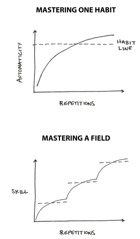
- Improvement is not just about learning habits, it’s also about fine-tuning them. Reflection and review ensures that you spend your time on the right things and make course corrections whenever necessary.
-
Perform annual review, in which reflect on the previous year, reflect on my progress by answering three questions:
- What when well this year?
- What didn’t go so well this year?
- What did I learn?
Answer three questions in the yearly Integrity Report:
- What are the core values that drive my life and work?
- How am I living and working with integrity right now?
- How can I set a higher standard in the future.
Never reviewing your habits is like never looking in the mirror. Periodic reflection and review is like viewing yourself in the mirror from a conversational distance. You can see the important changes you should make without losing sight of the bigger picture.
-
How to break the beliefs that hold you back:
The more scared an idea is to us — that is, the more deeply it is tied to our identity — the more strongly we will defend it against criticism.
One solution is to avoid making any single aspect of your identity an overwhelming portion of who you are.
“Keep your identity small”. The more you let a single belief define you, the less capable you are of adapting when life changes you. In other words, don’t be overconfident about your identity, Be acceptable to things.
-
When you spend your whole life defining yourself in one way and that disappears, who are you now?
The key to mitigating these losses of identity is to redefine yourself such that you get to keep important aspects of your identity even if your particular role change. I.E.
- Instead of saying “I’m the CEO”, say “I’m the type of person who builds and creates things”
-
Not “I’m a great soldier”, Yes “I’m the type of person who is disciplined, reliable, and great on a team”
Habits deliver numerous benefits, but the downside is that they can lock us into our previous patterns of thinking and acting — even when the world is shifting around us. Everything is impermanent. Life is constantly changing, so you need to periodically check in to see if your old habits and beliefs are still serving you.
-
A lack of self-awareness is poison. Reflection and review is the antidote.
Don’t let the Identity obstacle your belief. Be a Open Person.
Men are born soft and supple; dead they are stiff and hard.
Plants are born tender and pliant; dead, they are brittle and dry.
Thus whoever is stiff and inflexible is a disciple of death.
Whoever is soft and yielding is a disciple of life.
The hard and stiff will be broken.
The soft and supple will prevail.
人之生也柔弱,其死也坚强。草木之生也柔脆,其死也枯槁。故坚强者死之徒,柔弱者生之徒。是以兵强则灭,木强则折。
《道德经》– 老子