by Peter D. Schiff and Andrew K. Schiff
本书用一个假象的世界——小岛,讲述很多经济和社会现象的起源和影响,隐喻了很多现实中的事件和历史节点。从底层展示了经济的运行规律。
Good Book, but mixed with authors’ personal (something fair) feelings and emotions.
Chapter 1 经济一始
- Scenario 1
假设:在一个岛上(美索尼亚岛,后续11章会提及),三个人,每个人每天可以捕一条鱼,自给自足。没有货币、没有金融etc。
Life = Work + Consume
24h = Working + Leisure
Life = Fishing + Eating
生活相当于 <=> 工作(捕鱼) + 享受(吃鱼)。每天有24个小时,用一定的时间捕鱼,用剩下的时间吃鱼和享受Leisure。
-
Scenario 2
其中一个人A研制出了一个捕鱼工具——渔网。为此,他花了一天时间制作渔网,也挨了一天饿。
He takes the risks of starving, and create a “Capital 渔网” that can increase efficiency of working for long time.
“Tech” <-> Capital is created, which increase the efficiency.
他通过技术,制造了工具,提高了生产效率,可以在同样时间内,用渔网捕更多的鱼。但同时他每天仅需要吃一条鱼,那么用工具补的鱼可以被存起来变为 “Saving”;或者可以花更少的时间捕鱼,获得更多时间 Leisure
P.S. 以下均假设鱼Saving 不会变质,可以理解为是经济体的产出 Economic Outputs
Chapter 2 分享经济产出
-
小岛上的其他人也想要获得渔网,提升效率的工具。为此,他们可以选择
- 自己也挨饿一天制作渔网。可能有做不出渔网的方法。
但是由于 A 有储蓄,岛上的其他人可以向 A 借鱼吃,以免自己制作网的当天要挨饿。
-
但是对于 A 来说,他也有不同的 Options:
- No share saving.
不借给其他人吃,防止他们做不出渔网,或者还不上 A 借给他们的鱼。
这样 A 不会承担风险,但是经济体也不会增长。
-
Share saving ( with Interests or no interest ). 金融也因此产生了
把鱼借给其他人,同时收取“利息”,如:要求借出一条鱼,还两条(即利息是一条)。
- If 设置利息为0,那么就是再免费 share saving,
- If 设置利息不为 0,那么 charge interest,对方可能不还钱,那么 A 就亏了,也可以对方还钱,A 就挣了额外收入。
-
The cost of the interests is the game, and we do not talk about that further. just now.
- Invest the Saving.
A 还可以自己多制造更多的渔网,通过用现有渔网捕更多鱼 Saving,然后之后消费 Saving 制造更多的渔网。
A 可以开设自己的租鱼公司,将多余的渔网可以用于出租给其他人,挣租金。如果 A 制作渔网的技术无法被其他人学会,那么 A 的公司将能永远盈利。
- Other Options.
- No share saving.
- 我们假设,最终,无论中间经过了哪个 options,每个人都掌握了制作渔网的技术,因为模仿和抄袭的成本和难度远远比创新低。
-
每个人都获得了渔网,整个岛上所有人的生产效率都提升了,整个岛的 efficiency, 和 economic output 都提高了。
-
A 通过 tech,成为了岛上最初的富人,他可以为其他人提供有价值的东西。尽管此后所有人都有了 tech,他的 tech 变得不再特殊,无法再挣额外的利润。
-
在社会的角度,如果 A 有持续的获取利润的能力,或者如果 A 通过自己的利润持续压迫其他人,那么社会可能变得不稳定 instable。起义、变革,直到社会变得公平。The edge A have the ability of making profits is also a sociology game.
Chapter 3 Credit and Loan (Inserted)
In the case,A 有储蓄,可以选择投资 investment,把储蓄以贷款的形式投资出去,挣投资收益。
- 商业贷款:选择能还钱的借款人,有正向收益的项目等,都是为了保证贷款能收回。但是一旦外部力量以各种里有鼓励或者要求储蓄者借出款项,不考虑实际还款的可能性,那么贷款人就难免要承受较大的损失。
因为政府没有储蓄,只有个人才有,加入在政府的激励下,贷款流向了无法还款的个人和企业,那么个人的储蓄就被牺牲了。
-
消费贷款:消费贷是风险更高的贷款品种,因为 borrower 拿着钱去消费、度假了,没有用来获得正向现金流。Creditors 会因此承受不必要的风险,此时对 borrower 和 creditor 来说都是一笔负担。
-
应急贷款:为应对紧急情况而提供的贷款,可能 borrower 收不到这笔钱就完蛋,也可能 borrower 因为快完蛋了才需要这笔钱,收到了也得完蛋。但是当 borrower 处于不能,或者由外部因素让 borrower 不能完蛋的情况,可能不得不借。社会生死攸关之际,储蓄格外重要。
Chapter 4 How Economy Grows?
基于 Chapter 2 的结尾,每个岛民制造了渔网,大家捕鱼的效率都提升了,每天捕两条吃一条,岛上有了更多的 saving (Outputs, fishes)
他们花费 saving 的鱼,有更多时间开发新的设备,更强的捕鱼机器,etc
Technology boosts the Economy Growth.
Saving 储蓄发挥了作用:1. 给人们机会投资,用 tech 创造;2. 起到缓冲器的作用,应对自然灾害 crisis etc
Saving 创造了资本,资本使生产扩大成为了可能,所有储蓄起来的一美元对经济产生的积极影响要大于消费掉一美元。
Chapter 5 Service, Money, and Comparative Advantage
- 通过储蓄、贷款,人们有机会拓宽投资领域,扩张商业。
-
Service:当需要层次到达一定阶段,服务业应然而生(厨师,教培)
-
Money:为了满足不同人有不同的需求,如当制矛师向厨师买饭,而厨师不许要买矛时,货币(鱼)产生了,作为普适的交易媒介。
-
Comparative Advantages:在这个经济体中,人们发挥不同职能,如有的人擅长体力,他可以搬运更多的鱼,有更高的搬运效率,可以因此挣更多的钱。
-
Tech & Productivity:同时,有的人研发新的 devices,用车运输,而非人力运输,再次提高了生产效率 productivity,成本也因此降低了,利润提升了。
技术创新是个单向过程,除非人们失忆,否则生产效率提升会随时间越来越多。价格随时间降低。持续降低的价格还给人们更多空间储蓄
-
Employment: 劳动价值通常取决于劳动者所使用的资本,资本的便利,可以提升劳动的价值。如推土机推的土比人铲效率高得多。
- 劳动者在市场中可以扮演不同的角色:
- 制造渔网的人:创新者承担风险, start you own business
- 贷款买鱼网的人:加杠杆承担风险
- 为有渔网的人打工的人:打工人,稳定收入,风险低。
- 最低工资标准:政客通常表示,最低工资制度使员工获得了权益,但实际上也剥削了部分人获得工作的权力。如最低工资为 ¥8,而一个人的效率只值得 ¥6,那么他们会失业,员工选择的权力被剥夺了。政客提出的很多权益,如医保、产假等,实际上并未给员工提供好处,反而让员工失去了选择的权力(主动用自己工资去买这些权益的权力)。但是对政客来说,这么做可能意味着社会稳定性。
- Deflation 通缩:
作者认为通货紧缩是当今经济学中最成功的宣传册。经济学家认为通缩会对经济带来负面影响。
但是如作者此前观点,当efficiency提升,成本降低,价格会降低,那么必定会带来“通缩”。即,生产率的提升会促使价格下降。但这对经济体来说实际上是好事。
作者说,现代经济学错误的认为:消费促进经济增长,一旦通缩,人们不愿消费(价格会继续下降,spiral accelerate的负向),如果人们继续消费,价格下降的影响会减弱。
作者认为,起决定作用的不是消费,而是生产,不需要劝说人们消费,因为人类的需求永远不会得到猫族。如果人们不想要某样东西,那么一定是有理由的,要么商品不够好,要么买不起。
作者认为,政治家宣传通缩不好,是因为通缩是政治家的好朋友。
Chapter 6 What does Saving do?
-
Banker create a location, the bank, to accumulate indiviudal’s saving. 人们不愿意在家存放过多的鱼,于是把鱼存到银行。银行同时用吸纳的储蓄放贷,挣贷款利息。
- 储户:Banker 为储户支付利息,吸引他们把钱存到银行。
- 储户存的越久,Banker 给储户的利率就越高,因为 bank 获得了更稳定的鱼(钱),可以用来房贷款·。
-
放款:放贷款的时候,Banker 选择可靠的借款人,收取低利率。对风险高的借款人,收取高利率。
-
同时,如果鱼存量多,bank 会主动降低利率,因为 bank 承担损失的能力比较强。。
- 当储蓄过量,银行就不需要吸引新的储蓄,贷款利率也比较低,存款利率也比较低。这样也一定程度的抑制了储蓄。
- 一旦储蓄少了,银行想要吸引更多储蓄,给更多利率,同时流动性低,放贷款也要charge more interests。
- bank 作为中间金融机构实现了 equilibrium
-
Fund:
银行吸引相对稳定的钱,同时放贷给相对风险低的项目。但是市场中有不同的储蓄者(投资者)和项目。如:有点人能承担更多风险,想把鱼存下来,挣更多的收益。有点项目风险高,银行不愿意给放贷款。此时 Fund 出现了,吸纳 individual 有更高风险偏好的钱,把钱投给有更高预期收益,但是同时更高风险的项目。
- Fed:作为美国财政部的延申,负责制定基准利率,美国市场的利率结构都是建立在基准利率之上的。Fed 被授予这种权力,是为保证经济在繁荣期和萧条期能稳定运行。作者认为,这个机制存在两个缺陷:
- 需假设Fed 的人更了解市场,因此可以通过 ffr 来调整市场,
- Fed 的决策基于政治考量,而非经济因素,如:虽然低利率可以降低市场成本,但同时低利率还能帮时任总统获得更多支持度,因为刺激经济。
- 也因此,Fed 在 covid 之前大多时候都执行低利率的政策。这也推动美国市场长期保持低利率的状态,市场整体利率低,吸引不到储蓄(因为收益少),同时刺激了 loan (因为成本低)
Chapter 7 Infrastructure & Business
- Infrastrucutre Investment
人们意识到缺少基础设施(如没有水源,没路),岛民想寻求解决方案。
岛民决定融资建自来水厂,一方面解决当地缺水的问题,同时自来水厂的收益可以偿还贷款和利息。
基建投资 infrastructure 不光保证贷款能偿还,还提升了社会生产率,甚至推升出新的产业。
但是在项目发起时,投资者会权衡 opportunities cost,毕竟钱被用来投资自来水厂了,就不能用来投资其他项目了。这时投资不同项目就取决于投资者和gov(作为 social planner)的选择。
-
Business and Trading – (Comparative Advantages)
随着基建提升了的生产效率,新的产业也产生了。岛屿岛之间开始产生贸易,有些岛把自己过剩的产品出口,刚好有其他岛对此些产品有需求。每个人,每个岛和国家都会利用自己的优势实现利益最大化。
在自由贸易的情况下,在 international trading (岛与岛之间的交易)中,不同国家发挥自己的 comparative advantage
In reality, 在自由贸易中,政治考虑会使情况变得负责。如:自由贸易的反对者会为了保护美国的就业岗位,不受海外竞争影响,而限制低价商品进口,使本国产品在本国市场中任有竞争力。但是 in this case,反对者保护了供给侧,但是需求侧的消费者不得不承受更高的商品价格。Deadweight loss 产生了 (Economics 101)
Chapter 8 How the Government Forms
岛上最开始没有政府,但是当有外敌入侵时,individuals 独自往往难以面对,需要集体反馈。此时 gov 的重要性体现了,岛民决定组建一个对人民负责的政府,政府无权剥夺人们的自由。
岛民中需要选出 leader 来做决策。Assume 岛上的 gov中,由12名议员组成参议院,包括一名能行使行政权力的议长。
同时,为了维护社会稳定,也是为了保护岛民的生命权、自由权和财产权,参议院设立了一套法院体系来解决纠纷,同时成立警察小队执行法官的法令。
gov 建立国防用的基建。
岛民同意每年缴纳一些鱼作为税款,用于 gov 对整个岛的集体花费。
为保证税款不被乱用,人们制定宪法,明确了 gov 应有哪些权益。
法院系统设置了最高法法官,负责维护宪法的权威,并督促议员的行为。
一个政府成立了。
政府用税费雇佣了一些人,如灯塔看守、治安官、法官、海军桨手。大家明白如果没有向政府纳税的社会生产者,这些职位根本不会吃饭,如果没有生产者缴税,政府官员都吃不上饭。
Chapter 9 Evolution of the Govenment
社会保持平稳运行,基础设施完善,社会生产率逐渐提升。当需要层次达到一定阶段,劳动密集型产业的部分labour转去做服务业或者新型产业,如装修公司、巫医医院、剧院 etc。
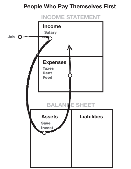
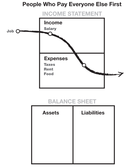
政府换届时,议员为了获得选票,演讲说要采取刺激的财政计划,支持经济发展。但是政府没有这么多钱(收入、税收、鱼),岛上的 saving 储蓄池不够政府完成支出计划,政府决定发行“鱼联邦储备券”,即可以用来去 bank 自由兑换鱼的纸币,一块钱 = 一条鱼。 政府控制了纸币的发行,就可以自由决定政府支出了。人们以后可以用纸币自由兑换鱼,也因此可以用纸币交易商品和服务。
鱼就像黄金,纸币就像美元。
Days later,政府超发了纸币用于财政支出,但是并没有足够的税收收入(真很正的鱼)来pay the fiscal expenditures,而是用纸币pay。市场的纸币越来越多,多过saving 鱼,导致不再是一块钱纸币能换一条鱼,而是每10块纸币只能换9条鱼。政府也意识到:当人们意识到银行美元足够的saving鱼用来兑换纸币,那么人们会去挤兑,run,去银行兑换鱼,政府就无法兑现 1-to-1 的承诺。
政府要做的,是让人们相信政府还有足够的saving 鱼,来满足兑换的关系。那么当政府超发纸币,人们就不会去挤兑。
In the story,政府研制了一种技术,可以把鱼拆分重组,用两条鱼制造三条鱼(鱼变小了,但是变多了)用来满足纸币兑换的需求。也因此,政府不再担心挤兑,开始肆意的印钱,欺骗人们有足够的 saving 做支撑政府做投资。
- In reality, 美联储早期建立布雷顿森林体系,指定35美元可以兑换1盎司黄金。但是美元不断超发,实际上美国储备的黄金并不能维持 1 盎司金 = 35 dollar 的关系。政府为了防止挤兑,就要用各种方式阻止提款,如限制兑换黄金的银行,禁止私人兑换黄金等。当时脱钩的关系不能阻止,直到一天,布雷顿森林体系瓦解。
Chapter 10 Fish Shrinks with Money Printed
政府不断用拼接鱼的技术来制造 saving (而不是真正的税收,或者output带来的saving),然后印钱,通过government spending 制造新的产业(无用,无意义的 bullsit jobs)用于保证就业,给人们发工资,维持社会稳定。这样的政府也获得了民众的支持,获得了选票,政府实力得到延续。
但问题是,鱼拼接技术,使 2条鱼 – 4条 – 8条 -16条 etc,虽然数量变多了,但是鱼变得越来越小、越来越小,直到人们意识到了问题。
因为纸币能换的鱼越来越小,物价必须上涨已弥补损失的营养价值。通胀问题产生了,尽管生产率提高会使物价下降,但是超发的货币 deduct that。物价上涨了。
简化这个过程,政府超发货币,为了满足社会问题,制造就业,创造了很多inefficient 无效的工作,给人们发工资,涨工资,但是真实产出(捕鱼数量没多,而是通过拼接变多了)并没有随超发货币的节奏,通胀问题产生了。物价上涨。
人们意识到了通胀问题越来越严重,鱼越来越小,通胀真正伤害的是需要养老的人,因为他们存的纸币能换鱼越来越小了,不能满足生活。
通胀问题越来越严重,人们选择把纸币花了买东西,而不是存钱,因为钱越来越不值钱了。通胀抑制了储蓄。储蓄少了,可以用来投资的钱也少了,新的产业在萎缩,企业削减成本,工人失业。社会不稳定的问题产生了。
此时新的政府选举来临,新的竞选者许诺要用 helicopter drop 的方式给人们发钱,满足消费需求。这种选举口号迎合了大众,当选,发钱。但是实际上 output resulted saving 没有提升,反而印了更多钱,通胀的问题更加严重了。
- In reality, espeically Keasian Economists 印钱来解决 recession 的问题,导致了 stagflation,通胀和失业同时出现。
人们认为失业时,需求会下降,物价会降低,导致通胀问题缓解,经济回到动态平衡的水平。但是人们没有意识到,失业,产业生产也减少了,供给减少了,物价也上升了。价格不会因为 unemployment 回落,因印钱导致的通胀不能缓解。
Chapter 11 External Player
作者假想:在一个新的经济体“中岛帝国”,经济体有更多的劳动力(人)labour,更集中的统治,人们捕鱼,上缴(缴税)。民众媒体只能吃到半条鱼,足以生活,但是国王和官员每天能吃到号线。中岛帝国没有储蓄、没有银行、没有信贷、没有企业,经济处于黑暗时代。经济没有持续发展。
中岛帝国的王得知美索尼亚岛后,打算学习银行、借贷和贸易系统,希望以此帮助自己的岛富裕。他认为货币是重要的因素,于是中岛帝国开始用鱼换美索尼亚岛的货币,因为货币可以保证随时在美索尼亚岛换取鱼,同时便捷交易。双方签订合约,中岛帝国定期提供鱼,换取美索尼亚岛的货币。
- 对于中岛帝国来说,他们用换取的货币,买美索尼亚岛上的产品。同时由于中岛帝国没有银行,他们只能把货币存在美岛挣取利率收益。
-
对于美索尼亚岛来说,中岛的购买力来买美岛的商品,为美岛提供了流动性。同时,中岛存入银行的鱼使可用的贷款大幅增加,岛上获得了额外的实物资本,已支撑岛内超发的货币。大量真鱼出现使货币换来的鱼的肉变多了,货币有了实物的支撑,物价上涨(通胀)的问题缓解了。
然而在中岛帝国,国王意识到,过多的税收,即让人们上交所有捕获,只留每天半条吃的量)阻碍了人们的生产动力。于是中岛开始向美岛买渔网,提高人们捕鱼效率。此前,每人每天捕一条,上交半条。现在每天捕两条,上交一条。win-win。
同时,一段时间后,中岛税收增加,持续用税收的鱼买美岛的货币,用货币买资本设备,持续扩大生产。
逐渐的中岛的企业家通过copy past,和创新,也产生了二产,有能力生产勺子、碗等基础产品。他们再把产品卖到美岛,换取货币。
Chapter 12 Evolution of Industrisation
中岛的储蓄(鱼)大量涌入美岛换取货币,储蓄被存入美岛银行,贷款利率随之降低,美岛企业家的投资热情也变得高涨。
- 美岛:由于中岛劳动力多,劳动成本低,美岛把大多捕鱼和制造业外包给中岛。而美岛发展和保留相对localised服务业,和附加值更高的产业。商业计划也更加青睐需要本地员工提供服务的项目,这些工作无法外包,且需要的资本少(轻资本、服务业),技术培训、艺术等。
-
中岛:中岛通过引入捕鱼技术,捕鱼效率大大提升,建造很多巨大捕鱼器(部分涉及通过copy past)。美岛告法院说中岛侵犯专利权,但是这个官司在中岛打不可能打赢。
中岛员工24小时工作,疯狂工作捕鱼,不发展服务业。但是对中岛的国王来说,人们整体忙于工作,甚至没有对服务业有需求的时间,社会稳定,不需要额外的改变。
中岛捕鱼效率高了,持续用捕的鱼,换美岛的货币。为美岛提供实物输血。中岛的人相信货币意味着产出和储蓄,而实际上这些被送往美岛的鱼被用来填补美岛超发货币的窟窿。
In reality,
过去20年,全球经济失衡(即美国贸易逆差)变为常态。相当于美国净获得了全世界的实物生产转为自己的消费,而全世界在用实物生产换美元。
美元储备货币的地位很大程度上导致了贸易逆差的扩大,如果没有全球经济体对美元的内在需求,任何国家都无法长期维持这种状态。
正常情况,贸金差额和货币价值应该处于一种动态平衡equilibrium的状态。一国的生产力更强,其他国家多这个国家的商品有需求,那么强势的贸易地位就会使一国的货币坚挺,弱势贸易地位的国家货币就会贬值。货币坚挺升值,产品的价格也变高了,需求少了,货币价值自然会降下来。
但是此前,中美货币之间的peg打破了这种关系,动态平衡的机制被破坏。
Chapter 13 The Breach of “Gold/Fish” Standard
即使有中岛定期的真鱼输入,美岛仍在超额印钱。开始有外岛的人质疑美岛货币的价值,质疑是否货币能兑换真鱼。于是人们开始去美岛银行兑换真鱼。
美岛银行显然没有足够的鱼来满足兑换,哪怕使用第10章的鱼拼接技术。
美岛政府决定打破鱼和货币的关系,暂停了银行兑换窗口。“鱼本位”瓦解。美岛货币的价值大幅降低。但是即使如此,美岛货币在岛与岛(国际)间交易的地位仍然存在。
In reality,这件事对应着Bretton Woods的瓦解。
Chatper 14 How Housing Price Increases?
银行不愿意投资服务业,业务风险高,而是更愿意寻找稳妥的项目,棚屋贷款,因为棚屋可以作为天热的抵押物。
此前,人们需要储蓄很多钱,然后一笔买棚屋。现在,人们通过贷款,直接买房,跳过了储蓄的时间。
然而银行还是会对人做挑选,富人更容易获得贷款,穷人被认为信用或还款能力较差,不那么容易被授予。
政府为了推动让更多岛民获得贷款,创立了“房利美”&“房地美”为棚屋贷款担保。有了担保,银行就不必担心贷款违约了,于是降低利率和放贷标准,更多贷款被制造出来。
银行开始允许“以小换大”贷款,低首付和棚屋利润免税政策。对棚屋的需求旺盛,推动供给侧更多的棚屋被生产出来,制造业的产业链被塑造,房地产吸收了越来越多的产能。
随着贷款刺激,棚屋价格开始上扬,棚屋的投资属性提升。Price Spiral Accelerately increased。
同时,中岛的钱也涌入美岛,进一步推动棚屋需求,价格进一步上涨。Bubbles Emerge
Chapter 15 Housing Bubble Collapses
由于岛民有限,对房屋的需求终究有尽头。
One day, 新房开始滞销。人们开始发现房屋的价格和价格、供需脱钩。
房屋数量多余人们的真是需求,人都开始想脱手,房屋价格开始大规模下跌。
消费者不再投资房屋,其他相关产业也陷入了困境。建筑工人、设计院、房处Sales,电器Sales纷纷失业。看似不相干的产业也同时收到了冲击。
小岛陷入了经济危机。
政府决定开展经济刺激援助计划。首先向“两房”注入资金(印钱),已保证房产有抵押,或者发消费券。政府希望持续放松信贷,提高市场对房产的需求,阻止价格下点。但显然由于供求失衡,这样做并没有效果。
同时,由于棚屋价格暴跌,人们觉得自己没有以前富裕,所有停止消费。
印钱显然无法从根部组织 bubble collapses 的问题,美岛政府希望寻求更多的鱼注入经济体,支撑超额印钱,已弥补房产市场。
于是美岛开始尝试卖自己的基建产业,如卖掉自来水系统,换取鱼。但美岛的反对派表示如此做会威胁到国家安全,让核心产业离开自己掌控。所以此做法也无法实现。
最终,政府只是提出了所谓“经济刺激援助计划”,但实际什么也没能做,不能改善经济环境。
Chapter 16 The Scenario Gets Even Worse
岛国房产行业崩塌,消费停滞。
新任政府通过“变革”的口号拿到了更多选票,再次扩大了经济刺激计划,并设计了其他新的计划,将新印刷的货币注入市场,增加助学贷款,开展超量基建建设并雇用人员运维,发展新能源等,
但是由于美岛已经没有鱼了,他们所有的开销背后都要依靠外国的资金支持。
经济层面,美岛人们可以有以下选择:1. 减少消费,用储蓄还债。2. 增大产量,卖掉多余的货物还债。3. 追加贷款,旁氏骗局,保持现有消费水平。
给予上述三种选择,前二都需要美岛人“吃苦”,而第三个option可以通过让外国人买新债来转嫁债务。于是美岛的官员选择了3。
Author’s View: 一国的经济不会因为人们的消费而增长,而是经济增长带动人们消费。
Chapter 17 IMF & PIGS
与美岛类似的剧情发生在了其他更“小”的岛,经济体量更小,但是没有美岛的货币在国际交易中的影响力。小岛经济逐步崩溃,经济危机。此时IMF,作为多国出资组建的机构,为小岛提供了大量的美岛货币(目前仍被视为最可靠的货币),希望帮助小岛度过危机。
IMF提供的援助贷款利息很低,但仍需要真是的鱼(output)用于到期偿还。同时,IMF强制小岛政府接受一系列的“刚性”计划,包括提高税收、减少政府支出等。此计划被当地居民强烈抵制,因为居民觉得自己的岛屿被不怀好意的外岛人控制了。
Another Real-world Scenario
2010年,PIGS时陷入债务危机,他们作为欧盟成员,国家维系着丰厚的社会保障体系,但是国家债务水平远超本国经济发展能力。
政府想用量化宽松政策来修复萎靡的经济,就好像企图用汽油去救火,汽油越多,火势越旺。
Chapter 18 What Does/Did CB do?
美岛QE,CB开始Operation Squish的操作,将长期联邦贷款替换短期的,将还款期限延长。虽然始终没有真是的鱼(output)做支撑,但是民众被“无限期债”的计划带来了正向的预期,该计划再次短期抬高了房价,人们追求趋势再次投入资金。然而,CB的操作并没有为市场带来真正的output,当房价暴跌的时候没有人幸免。
In reality,
- at the end of 2008, CB conducted QE, purchasing about 2 triilion USD debts (Open Market Operation).
-
2010Q1, after CB reduces purchasing, the stock market collasped. CB conducted the second round of QE , and was coined as “Monetaisation of those Debts”
- 2011Q2Q3, after the end of the second round QE, Fed did Operation Twist, replacing short-term debt with long-term ones. That conduction results in the booming housing market, but is less helpful for the “real” term economy. Stock price hiked but employment went worse.
Chapter 19 The End
中岛逐步打造自己的内循环经济体系后,逐步发现不再需要美岛发行的货币,逐步与美岛脱钩。于是中岛逐步减少向美岛输送output,用来换货币。
中岛继续捕鱼、制造商品、储蓄,这些都是促进其经济增长的因素,中岛也未陷入经济危机。
而美岛因为过度发展服务业和金融业,国内逐渐丧失了制造能力。更多的货币,和更少的output,通胀更加严重。钞票贬值、商品稀缺、物价飞涨。
中岛带着大批的鱼&货币来美岛采购,买基础设施买固定资产,然后离开…
In reality,
The author summarised that 政府总会因为入不敷出而陷入困境,一旦loss累计到一定程度,政府就会面临艰难的选择。
- Option 1. 提高税收。但是人民不喜欢税收,高税收会抑制生产、降低经济活力。税收过高,人们会停止巩固走,甚至发生暴乱。
- Option 2. 削减政府开支。但是这种做法往往会有更多人(利益相关方)反对。
- P.S. 政客为了赢得选举做出无数承诺,而选民从不考虑纳税人是否为这些承诺买单。
- Option 3. 政府拒绝缓债,如果债权人是外国人,那么从政治上,与其增加税收并掠夺国人利益,不如失信于外国人。
- 对于政客,拒绝还债往往令难堪,因为需要承认自己没有偿付能力。为了避免这个情况,政客索性选择印钱,引起通胀,使债务贬值,还债。但以通胀作为代价往往是最次的选择。