The current mostly used Solow model always have a depreciation term, and thus the law of motion becomes, \(\dot{K}=I-\delta K\).
The mainstream model has different assumptions about the production function as well. For example, technological progress is generally added. 1. \(Y=AF(K,L)\) in which technology is exogenous, and it could be called Hicks-neutral; 2. \(Y=F(K,AL)\) that can represent the efficient workers, labour-augmented, or Harrow-neutral; 3. \(Y=F(AK,L)\) in which the technological progress is capital augmented.
Applying for example the labour-augmented technology and \( \frac{\dot{A}}{A}=g\) , we can simply solve the Solow model as the following,
$$k=\frac{K}{AL}$$
$$ \frac{\dot{k}}{k}= \frac{\dot{K}}{K}- \frac{\dot{A}}{A}- \frac{\dot{L}}{L} $$
$$ \frac{\dot{k}}{k}= \frac{sY-\delta K}{K}- \frac{\dot{A}}{A}- \frac{\dot{L}}{L} $$
$$ \frac{\dot{k}}{k}= \frac{sY}{K}-\delta-g- n $$
$$ \dot{k}=sy-(\delta+g+n)k $$
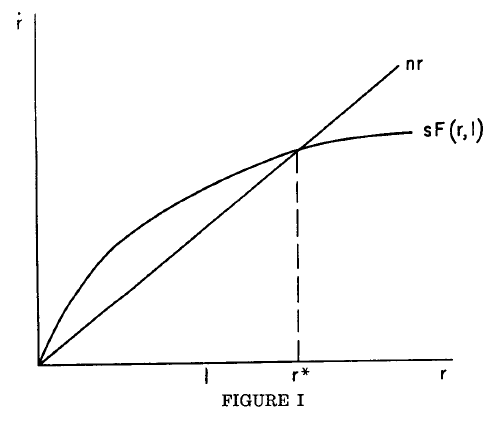
, where \(y=\frac{Y}{AL}\) and \(\frac{K}{AL}\) represent the output/capital per efficient works. Therefore, if \(\dot{k}=0\), then \(sy=(\delta+g+n)k\).
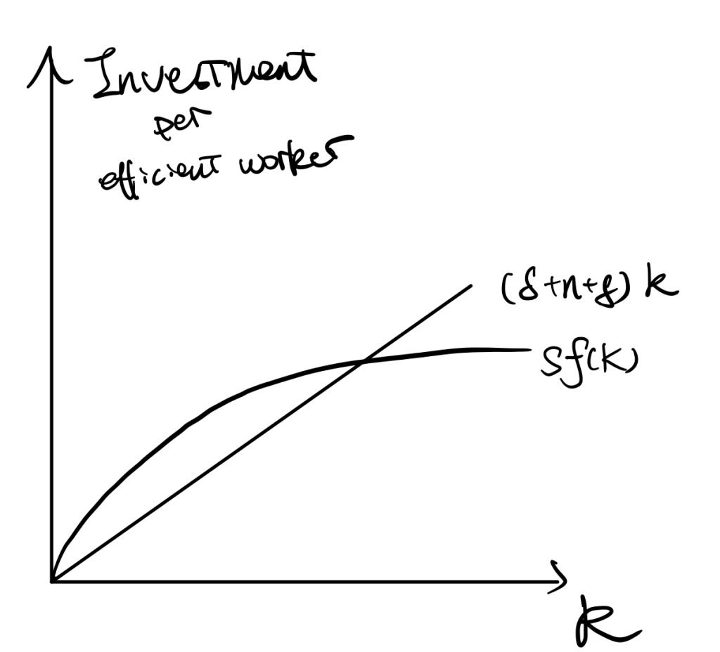
The stable point of k is \(k^*\) in which \(sf(k)=(\delta+n+g)k\).
We always the Cobb-Douglas function to represent the production function, because it satisfies CRTS, increasing and diminishing assumptions, and the Inada conditions (\(\lim_{k\rightarrow0}f'(k)=\infty; \lim_{k\rightarrow \infty}f'(k)=0\), Inada, 1963 ).
In the following, we would all analyse the model using efficient works to do analysis.
Balance Growth Path
All the following is assuming the economy is at the steady state or stable point.
For \( \frac{\dot{K}}{K} \),
$$ k=\frac{K}{AL} $$
By taking logritham,
$$ ln(k)=ln(K)-ln(A)-ln(L) $$
By taking differentiation and set \(\dot{k}=0\) (based on our previous derivations of finding the steady state condition).
$$ \frac{\dot{K}}{K} = \frac{\dot{A}}{A} + \frac{\dot{L}}{L} $$
$$ \frac{\dot{K}}{K} = g+n $$
For \( \frac{\dot{Y}}{Y} \), similar as the original Solow’s one.
$$ln(Y)=ln(F(K,AL))$$
Differentiate w.r.t. \(t\),
$$ \frac{\dot{Y}}{Y}=\frac{ \dot{K}F_1’+\dot{A}LF_2’+ A\dot{L}F_2′ }{F(K,AL)} $$
By Euler’s Theorem to the demoninator (see math tools),
P.S. differentiate \(tY=F(tK,tAL)\) w.r.t. \(t\), then we get \(Y=F’_1 K+F’_2 AL\).
$$ \frac{\dot{Y}}{Y}=\frac{ \dot{K}F_1’+\dot{A}LF_2’+ A\dot{L}F_2′ }{ F’_1 K+F’_2 AL } $$
Devide both numerator and demoninator by \(KAL\),
\frac{\dot{Y}}{Y}=\frac{ \frac{\dot{K}}{KAL}F_1’+\frac{\dot{A}L}{KAL}F_2’+\frac{ A\dot{L}}{KAL}F_2′ }{ \frac{F’_1 K}{KAL}+\frac{F’_2 AL}{KAL} }
\frac{\dot{Y}}{Y}=\frac{ \frac{\dot{K}}{K}\frac{F_1′}{AL}+\frac{\dot{A}}{A}\frac{F_2′}{K}+\frac{ \dot{L}}{L}\frac{F_2′}{K} }{ \frac{F’_1 }{AL}+\frac{F’_2 }{K} }= \frac{ \frac{\dot{K}}{K}\frac{F_1′}{AL}+(\frac{\dot{A}}{A}+\frac{\dot{L}}{L})\frac{F_2′}{K} }{ \frac{F’_1 }{AL}+\frac{F’_2 }{K} }
\frac{\dot{Y}}{Y}= (n+g)\frac{ \frac{F_1′}{AL}+\frac{F_2′}{K} }{ \frac{F’_1 }{AL}+\frac{F’_2 }{K} } = (\frac{\dot{K}}{K})\frac{ \frac{F_1′}{AL}+\frac{F_2′}{K} }{ \frac{F’_1 }{AL}+\frac{F’_2 }{K} }
$$ \frac{\dot{Y}}{Y}=n+g = \frac{\dot{K}}{K} $$
For \( \frac{\dot{y}}{y} \), (as \(y=\frac{Y}{AL})
$$ln(y)=ln(Y)-ln(A)-ln(L)$$
$$ \frac{\dot{y}}{y}= \frac{\dot{Y}}{Y}- \frac{\dot{A}}{A}- \frac{\dot{L}}{L} =(n+g)-n-g $$
$$ \frac{\dot{y}}{y} =0$$
Similarly, for per capita terms,
For \( \frac{\dot{K/L}}{K/L} \), per capita capital,
$$\frac{\dot{K/L}}{K/L}=\frac{ \frac{\dot{K}L-K\dot{L}}{L^2} }{K/L}$$
$$\frac{\dot{K/L}}{K/L}=\frac{\dot{K}L-K\dot{L}}{KL}= \frac{\dot{K}}{K}- \frac{\dot{L}}{L} $$
\frac{\dot{K/L}}{K/L} =(g+n)-n=g
For \( \frac{\dot{Y/L}}{Y/L} \) (per capita output) we apply the same transformation as K/L,
\frac{\dot{Y/L}}{Y/L}= \frac{\dot{Y}}{Y}- \frac{\dot{L}}{L} =g
In summary, the BGP is a situation in which each variable of the model is growing at a constant rate. On the balanced growth path, the growth rate of output per worker is determined solely by the rate of growth of technology.
P.S. Technology Independent of Labour And Capital
Applying for example the Type 1 case and \( \frac{\dot{A}}{A}=g\) , we can simply solve the Solow model as the following,
We would not use capital per efficient worker here, because labour is not technology-augmented by assumption. Instead, we simply assume capital per capita, \(k=\frac{K}{L}\). We can easily get the relationship,
\frac{\dot{k}}{k}= \frac{\dot{K}}{K}- \frac{\dot{L}}{L}
By setting \(\dot{k}=0\), we can find \( \frac{\dot{K}}{K}=\frac{\dot{L}}{L}=n \), which is same as Solow’s original works.
However, the difference is when we deal with the output. As the output is now \(Y=AF(K,L)\), so the changes in outputs (numerator) are,
$$ \dot{Y}=\dot{A}F(K,L)+AF’_1\dot{K}+AF’_2\dot{L} $$
We expand output per se (demoninator) by Euler’s Theorem \(Y=AF’_1K+AF’_2L\) (A is now outside the production function), and then calculate the percentage changes of outputs,
$$ \frac{\dot{Y}}{Y}=\frac{ \dot{A}F(K,L)+AF’_1\dot{K}+AF’_2\dot{L} }{ AF’_1K+AF’_2L } $$
Devided both demoninator and numerator by AKL,
$$ \frac{\dot{Y}}{Y}=\frac{ \dot{A}F(K,L) }{ AF(K,L) }+\frac{\frac{F’_1}{L}\frac{\dot{K}}{K}+\frac{F’_2}{K}\frac{\dot{L}}{L} }{ \frac{F’_1}{L}+\frac{F’_2}{K} } $$
$$ \frac{\dot{Y}}{Y}= \frac{\dot{A}}{A}+ \frac{\dot{L}}{L}=g+n $$
Saving Rates
We now consider first how does changes in the saving rate affect those factors.
The determinants of saving rate are, for example, uncertainty or decrease in expected income, and required pension rate.
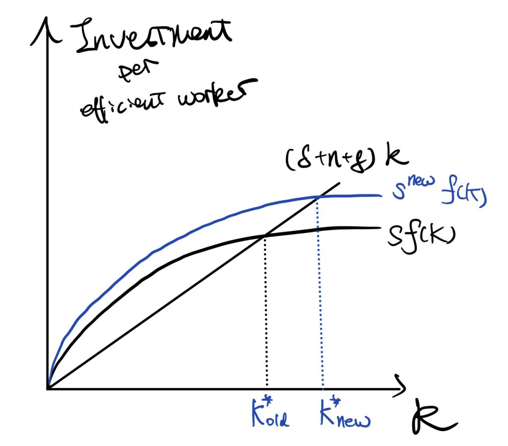
See the following figures,
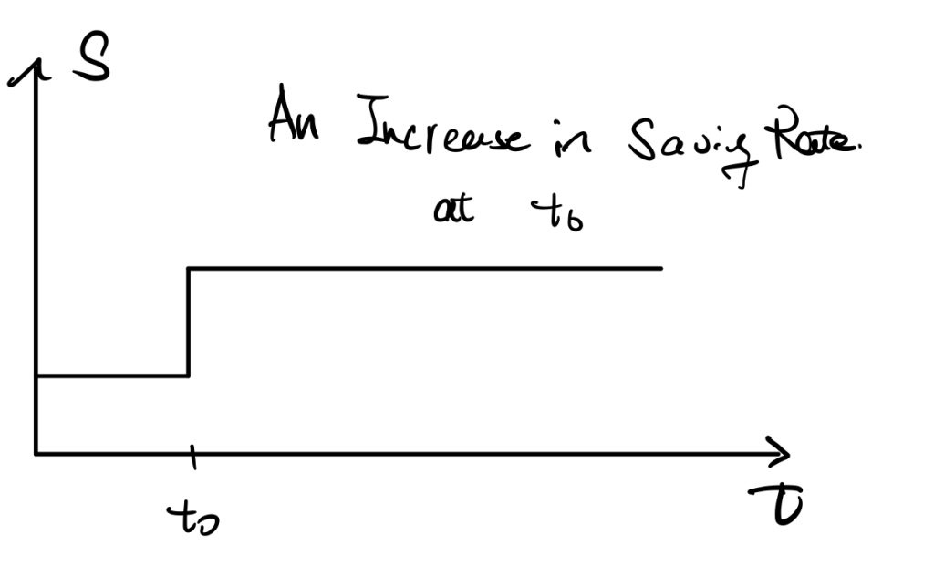
An increase in the saving rate would result in an increase in the investment curve. \(\dot{K}=I-\delta K\) tells that there would be a huge increase in \(\dot{K}\) initially, and by the shape of production function, the difference diminishes until achieving the new stable point \(k^*_{new}\).
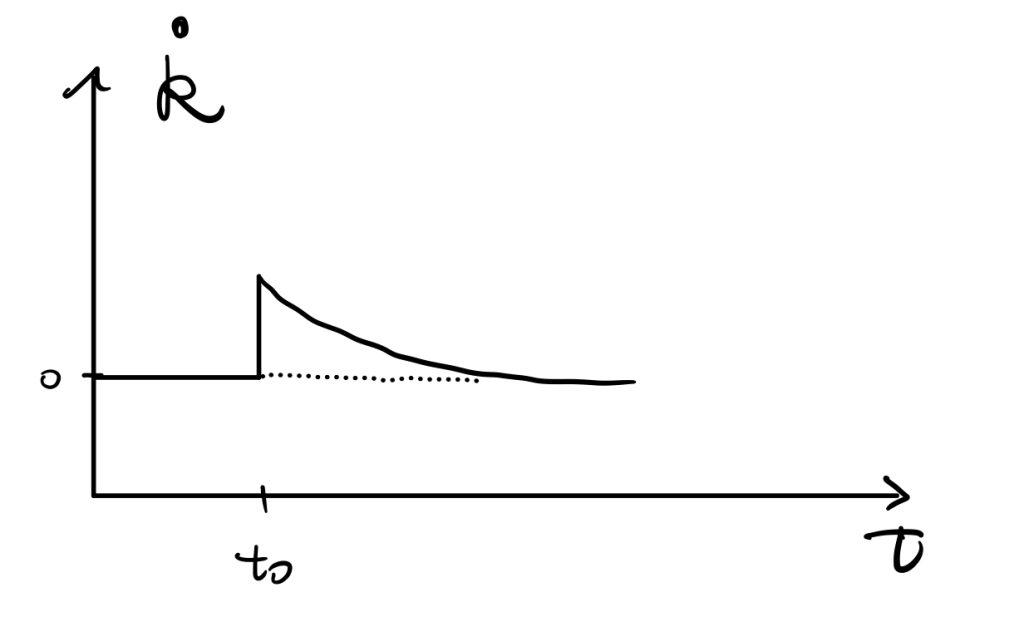
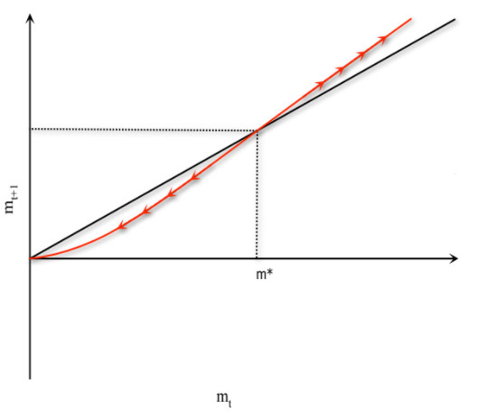
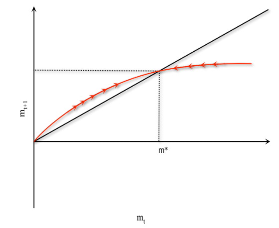
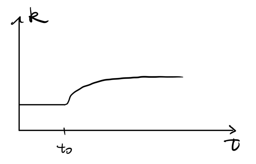
As \(\dot{k}\) is a derivative of \(k\) w.r.t. \(t\), we can easily get the time path of \(k\) as the following,
Another important factor is the growth rate of output per capita,
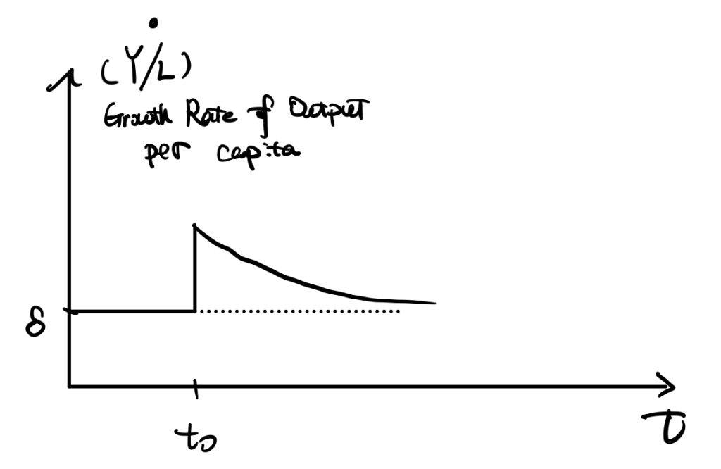
Also \(ln(Y/L)\),
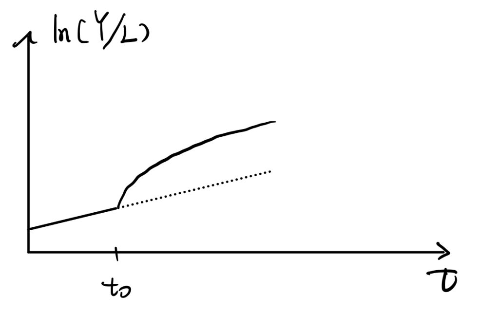
For this one, we can prove that the slope of \(ln(Y/L)\) is \(\dot{ln(Y/L)}=\frac{\partial}{\partial t}[ln(Y)-ln(L)]=(g+n)-n=g\), so it grows constantly at rate “g” before \(t_0\). Later growth rate of Y jumps makes the slope of \(ln(Y/L)\) increases, but \(ln(Y/L)=g\) when achieves a new steady state and \(ln(Y/L)\) keeps growing at “g” in the long run.
The Speed of Convergence
Way 1
We follow our Solow model with labour-augmented technology. The time path of changes of capital per efficient works is,
$$ \dot{k}=sy-(\delta+n+g)k$$
$$ \dot{k}=sy-(\delta+n+g)k$$
At the steady state, \(\dot{k}=0\), so \( sy-(\delta+n+g)k \). We then plug in the Cobb-Doglas production function and denote \(y=\frac{Y}{AL}=\frac{K^{\alpha}(AL)^{1-\alpha}}{AL}=k^{\alpha}\), we can find the \(k^*\),
$$ k^*=(\frac{s}{\delta+g+n})^{\frac{1}{1-\alpha}} $$
And get the path of k,
$$ \frac{\dot{k}}{k}=sk^{\alpha-1}-(\delta+g+n) :=G(k)$$
To find the speed of convergence, we would focus on the time path of k around \(k^*\). Or approximate the time-path by taking first-order Taylor expansion around \(k^*\) to approximate,
$$ G(k)\approx G(k^*)+G'(k^*)(k-k^*) $$
As \(G(k^*)=0\) by our proof of steady state condition, thus,
$$ G(k)\approx (\alpha-1)s {k^*}^{\alpha-1}\frac{k-k^*}{k^*} $$
We plug the steady state \(k^*\) back into the above equation and get,
$$ G(k)=-(1-\alpha)(\delta+g+n)\frac{k-k^*}{k^*} $$
Therefore, we find the mathematic expression of the convergence speed, \( (1-\alpha)(\delta+g+n) \). It is the measure of how quickly k changes when k diviates from \(k^*\). Also, we find that the growth rate \( G(k)=\frac{\dot{k}}{k} \) depends on both the convergence speed and \( \frac{k-k^*}{k^*} \), which is how far k deviates from its steady state level.
Take also a Taylor expansion to \(ln(k)\) at \(k^*\), we would get,
$$ G(k)=-(1-\alpha)(\delta+g+n)(ln(k)-ln(k^*)) :=g_k$$
Then, to find the convergence speed of outputs, we apply \(y=k^{\alpha}\) and take logritham \(ln(y)=\alpha ln(k)\). Differentiate w.r.t. \(t\),
$$ \frac{\dot{y}}{y} =\alpha\frac{\dot{k}}{k} $$
$$ g_y:=\frac{\dot{y}}{y} =\alpha( -(1-\alpha)(\delta+g+n)(ln(k)-ln(k^*))) \\= -(1-\alpha)(\delta+g+n)(ln(y)-ln(y^*)) $$
So we get \(g_y=\alpha g_k\), and \(\beta= (1-\alpha)(\delta+g+n) \) is the speed of convergence. It measures how quickly \(y\) increases when \(y<y^*\). The growth rate of y depends on the speed of convergence, \(\beta\), and the log-difference between \(y\) and \(y^*\).
Way 2
We take first order Taylor approximation to \(f(k)=\dot{k}\) around \(k=k^*\).
$$ \dot{k} \approx \dot{k}|_{k=k^*}+\frac{\partial \dot{k}}{\partial k}|_{k=k^*}(k-k^*) $$
By definition of steady state condition, the first term of RHS is zero. So,
$$ \dot{k}\approx -\lambda \cdot (k-k^*) $$
We denote \(-\frac{\partial \dot{k}}{\partial k}|_{k=k^*}\:=\lambda\) as the speed of convergence. As \(\dot{k}=sy-(\delta+g+n)k=sk^{\alpha}- (\delta+g+n)k\), so,
$$ \lambda=-s\alpha {k^*}^{\alpha-1}- (\delta+g+n) $$
Plug \(k^*\) into, we get,
$$ \lambda=(1-\alpha)(\delta+g+n) $$
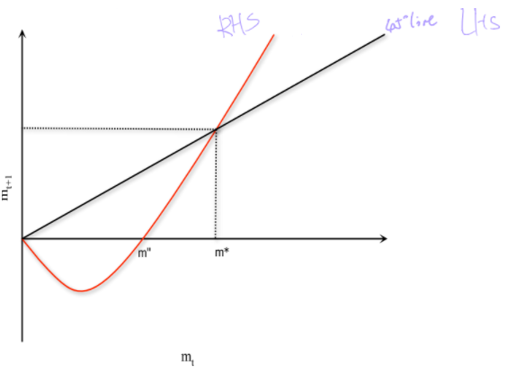
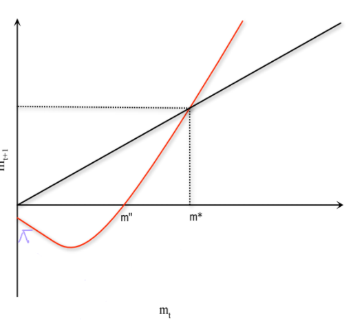
To see why we denote \(\lambda\)as the speed of convergence, solve the differential equation, \( \dot{k}\approx -\lambda \cdot (k-k^*) \), by restrict time from 0 to t.
$$ \dot{k}=\frac{\partial k}{\partial t} \approx -\lambda \cdot (k-k^*) $$
$$ \frac{1}{k-k^*} dk=-\lambda dt $$
$$\int_{k(0)}^{k(t)} \frac{1}{k-k^*} dk=\int_{0}^t -\lambda dt $$
$$ [ln(k-k^*)]|^{k(t)}_{k(0)}=-\lambda t|_0^t $$
$$ ln(k(t)-k^*)=-\lambda t|_0^t+ ln(k(0)-k^*) $$
Finally,
$$ k(t)=k^*+e^{-\lambda t}[ k(0)-k^* ] $$
Or in other form,
$$ ln(\frac{k(t)-k^*}{k(0)-k^*})=-\lambda t $$
Solow Residuals
Recall our labour-augmented production function, \(Y(t)=F(K(t),A(t)L(t))\).
$$ \dot{Y}=\frac{\partial Y}{\partial t}=F’_1\dot{K}+ F’_2\dot{A}+ F’_2\dot{L} $$
$$\frac{ \dot{Y}}{Y}=\frac{\partial Y(t)}{\partial K(t)}\dot{K(t)}+ \frac{\partial Y(t)}{\partial L(t)}\dot{L(t)}+ \frac{\partial Y(t)}{\partial A(t)}\dot{A(t)} $$
Then, applying the replacement equation into the above equation,
$$ \frac{\partial Y(t)}{\partial L(t)}=\frac{\partial Y(t)}{\partial A(t)L(t)}\cdot A(t) $$
$$ \frac{\partial Y(t)}{\partial A(t)}=\frac{\partial Y(t)}{\partial A(t)L(t)}\cdot L(t) $$
Then we get,
$$ \frac{ \dot{Y}}{Y}=\frac{Y(t)}{K(t)}\frac{\dot{K(t)}}{K(t)}\frac{K(t)}{Y(t)}+ \frac{Y(t)}{L(t)}\frac{\dot{L(t)}}{L(t)}\frac{L(t)}{Y(t)}+ \frac{Y(t)}{A(t)}\frac{\dot{A(t)}}{A(t)}\frac{A(t)}{Y(t)}\\=\epsilon(t)_{Y,K}\frac{\dot{K(t)}}{K(t)}+ \epsilon(t)_{Y,L}\frac{\dot{L(t)}}{L(t)}+R(t) $$
,where we denote \(R(t)\) as the Solow Residuals.
$$ R(t) = \frac{Y(t)}{A(t)}\frac{\dot{A(t)}}{A(t)}\frac{A(t)}{Y(t)} $$
Solow Residuals represent the residuals unexplained by growth of capital and labours.
Golden Rule Saving Rate (Phelps)
To be continued.