Three monetary regimes, aiming to avoid or mitigate the liquidity trap, are introduced here. They are Inflation Targeting (IT), Price Level Targeting (PLT), and Nominal GDP Targeting (NGDPT).
A brief summary is that NGDPT performs better than PT ( in terms of dealing with the liquidity trap), which in turn performs better than IT.
Before doing the analysis, we modify the model a little bit that makes the price to be “somewhat flexible”.
$$ \bar{p}_t=\frac{m_t}{y_t} $$
In that, if not in the liquidity trap, we assume \( p_t\geq \gamma \bar{p_t}\), with \(\gamma \in (0,1)\). (we previously assume \(p_t\geq \bar{p_t})\).
Let the inflation target be \( \frac{p_{t+1}}{p_t}=1+\pi\), then our Euler equation becomes,
$$ u'(\hat{y})=\beta \frac{1}{1+\pi}u'(y’) $$
Therefore, \( \uparrow \pi \Rightarrow \uparrow RHS \Rightarrow \uparrow LHS \Rightarrow \uparrow \hat{y}\). Increase in inflation would raise the current output.
Implication:
The fall in current output in the crisis is less severe (as \(\uparrow \hat{y}\)).
The economy is less likely to fall into a liquidity trap in the first place, because people know inflation in the future, so they will not likely be strucked in the liquidity trap, coz increasing demans in current time) High inflation means money loses value quickly, and thus agents are reluctant to save using cash.
Price Level Targeting
With the price level targeting, the CB aims to keep the price level on a certain path. This means if the CB fails to meet the target, it will catch up in teh later period. For example, if the price level is 100 at period \(t\), and the CB’s price level target is 2%, then the price level in period \(t+1\) should be 102. However, if the CB fails to do that in \(t+1\), then in \(t+2\) the CB should catch up and keep the price level to be 104.
In that, the CB follows \( p_{t+1}=(1+\mu)\bar{p_t}\), where \( \bar{p_t} \) is the “normal times price level”, and \(\bar{p_t}=\frac{m_t}{y_t}\).
If \(\pi=\mu\), then the RHS of the second Euler equation is smaller, and thus \(\hat{y_{PLT}} > \hat{y_{IT}}\). (easy to show in maths by assuming the isoelasicity utility function).
NGDP Targeting
With NGDPT, the CB aims to keep nominal GDP on a certain path. For example, aiming to increase NGDP by 2% per year. A failure in one period means a cathcing up in the next period.
Since \( \frac{y’}{y_t}<1 as y'<y_t, and \gamma \in (0,1)\), so RHS is even smaller than that of the PLT Euler equation. Therefore, \(\hat{y_{NGDPT}}\) is even greater than the \(\hat{y_{PLT}}\). That implies that the cirsis would be less severe for a given \(y’\).
In a standard open market operation, \(d_{t+1}\) (and \(b_{t+1}\)) would fall, and \(m_t-m_{t-1}\) would rise by the same amount. CB or Gov buy back debts and pool money into the market, so the net debt outstanding decrease and amount of money oustanding increase.
Nothing really changes in the Euler equation for private sectors. In other words, \( \hat{y} \) is still decresed from \(y_t\), and is not affected by changes in \(m_t\). \(p_t=\frac{m_t}{y_t}\), partially because \(p_t\) is predetermined already.
Intuitively, private sectors know the money would be taxed back, so they just hold the extra money (hoard them), and will pay them back as future tax payments. (That’s is the way to make the Euler equation hold). The excess cash holding would not bring an increase in future consumption, because that cash is all for future taxes. Consider the Ricardian Equilibrium.
P.S. that could be a Pareto-improvement to coordinate on spending.
As Keynes called “Pushing on a string”. Even if CB drops money from helicopters, the money would not be spent and would be hoarded. Therefore, no real impacts on the economy.
As shown in the figure, an increase in the money supply (monetary base) would result in people holding more money (excess reserve). At the moment in around 2008, the effective federal fund rate hits zero, liquidity traps started. Injecting more money (increasing the money supply) cause excess cash holding, instead of current output increase.
Forward Guidance
Forward guidance means committing to change things in the future (, with perfect credibility).
Assume that he government commits to expand money supply from /(m/) to /(m’/) in period \(t+1\) onward. Also, assume not in the liquidity trap in \(t+1\), (\(v_{t+1}=1\)). So the price level at \(t+1\) would be,
An estimated decrease in future outputs would increase \(y’u'(y’)\). However, a permanent increase in \(m’\) to keep the equation unchanged.
Forward Guidance differs from the conventional monetary policy because an extra amount of money would not be taxed back. The central bank “commits to act irresponsibly” in the future. Also, the conventional monetary policy emphasises the current money supply, but forward guidance states the future. People will know that there is no need to pay extra tax back in the future.
The is no clear downward trend of the real output while increasing money supply after getting into the liquidity trap. The market in the US implies that public sectors react to the expected decrease in future output by increasing the money supply in a long period (equivalent to the forward guidance), therefore the real output at the current period does undergo a significant decrease.
See Krugman (1988) and Eggertsson and Woodford (2003).
Here, we consider a production economy instead of an endowment economy. In this way, instead of being endowed with \(y_t\) units of the output good in each period, agents are endowed with one unit of time and they choose an inelastic supply of working.
Firms are perfectly competitive and produce output according to \(y_t=z_t l_t\), where \( z_t\) donates labour productivity and \(l_t\) the amount of labour hired.
A representative firm’s optimisation problem is then given by
$$ \max_{l_t} p_t z_t l_t- \tilde{w_t}l_t $$
F.O.C.
$$p_t z_t =\tilde{w_t} $$
The first-order condition tells that nominal wage stickiness leads to price stickiness. Given wages, \(\tilde{w_t}\), a fall in prices would reduce profits, and firms would shut down their businesses (by perfect competition assumption).
However, if prices and wages fell in equal proportion, firms would still like to hire equally many works. And the fall in prices would boost demand. P.S. the real wages keep constant.
Intuition: Firstly, as prices fall, goods get cheaper. So even 80 of spending can buy100 worth of goods. Secondly, as wages also fall, real profits are unchanged, and firms are willing to meet the additional demand. Finally, the positive impacts on \(y_t\) could offset the negative of it (from underestimated future outputs).
\( \quad \downarrow P \Rightarrow \downarrow W \Rightarrow\) unchanged profits and increase outputs
Quantitative Easing
In the open market operation, the CB purchases short-term government bonds (3-month T-bill). By QE, the CB purchases assets with longer maturity and credibility, see The Fed’s Balance Sheet, e.g. MBS.
The idea of QE is to decrease the interest rate once the short term rate is already zero, and also pool money into the market. In the recession, short term bonds’ nominal interest rates are already zero, but long term bonds may not. Thus, by purchasing long-term bonds, yields are pushed downward (real interest rate falls), and stimulate the economy. (Similar to the non-arbitrage theory). Long-term assets are equally valuable as short term assets at any horizon. In the liquidity trap, short term assets are equally valuable as holding money, so long term assets are perfect subsites to money as well (consider including liquidity premium and risk premium).
In the model with Cash in Advance and short long term assets, we consider include
A short term asset (one period) \(b_{t+1}^1\).
A long term asset (two periods), \(b_{t+1}^2\).
The price of the short-term asset is denoted \(q_t^1\), and pays out one unit of cash in period t+1.
The price of the long-term asset is denoted \(q_t^2\), and pays out one unit of cash in period t+2.
Equivalent to \( Return\ of \ LongTerm=Ro\ ShortTerm=Ro\ Cash\).
Long-term bonds are traded at arbitrage with short-term bonds which are traded at arbitrage with money.
Recall that the purpose of QE is to reduce the return on long-term bonds but that cannot be done.
If in the liquidity trap, \( x_{t+1}=0, \mu=0, i_t=0 \Rightarrow \frac{1}{q_t^1}=1 \Leftrightarrow \frac{q_{t+1}^1}{q_t^2}=1 \).
In the figure, the green curve represents QE (Fed Balance sheet). During the 2008 financial crisis and Covid-19, the Fed purchase assets (MBS and Long-term T bonds) and pay with money, in order to release liquidity into the market.
The word “real” means the real term in contract with the word “monetary”. Therefore, the real business cycle is not about the monetary policy, but about the negative supply shock. The RBC theory explains most of the business cycle in human history.
Examples
For example. in the early agriculture society, agriculture consists most of GDP. If extreme weather condition happens (the real shock), then there are bad harvests and bad outputs for almost all economy. People have less to eat, and an economic recession emerges. In the modern economy, outputs are more diversified. Another is that in the 1973 oil crisis, the OPEC oil embargo induced the oil price increase. The increase in oil prices made production costs increase for other goods and services, and led to an overall recession. A recent example is a crisis in Brazil. A decrease in commodity prices hugely reduced incomes (net export). Also, the Brazilian government became erratic and unpredictable (no clear target and no credible), bringing further risks to the Brazilian economy.
Shocks
Examples of shocks are,
Technology schoks
Policy shocks: Fiscal policy & Monetary shocks
Political shocks: changes in polical party
Expectations shocks: animial spirits
Natural disaster
Propagation mechanisms
Two Propagation mechanisms are here, the labour propagation mechanism and the intertemporal one. See notes.
Potential Solutions
Try to avoid the problem in the first place. For example, if the oil price is expected to increae, then invest in other alternative energy to decreae the effects of oil price increase on production costs. In other word, diversity the production costs and make the production process not rely too much on oil.
Make the economy more flexible and can be adjustable to negative supply shocks quickly.
Problems
It do not explain all business cycles, which are not caused by supply shocks. For example, a lot busienss cycles are about monetary polcy, banking, and credit.
It does not explain why unemployment rate is so high in labour economics.
In short, before the RBC model, macroeconomic studies mainly focus on the IS-LM and AD-AS. The building up of RBC solves the problem that macroeconomic study did not have a solid microeconomic background.
RBC model is like a new classical model with shocks, based on the key assumption that markets are perfectly competitive. Then, market players maximise their utility subject to certain constraints. Through the RBC model, we can get the co-movement of outputs, labours and capitals. Market fluctuations are caused by shocks. Without shocks, the markets are in equilibrium condition over time, because markets are competitive. Meanwhile, money is not included in the RBC model, so all factors are in real terms.
The first oil crisis started with the oil embargo proclaimed by OPEC.
OPEC: Oil exporting nations accumulated vast wealth due to the price increase. US: the oil price increase induced the recession, inflation, reduced productivity, and low economic growth.
Whyt did Keynesian economics fail in the 1970s?
According to Keynesians, the growth in the money supply can increase employment and promote economic growth. Keynesian economists believe in the Philips relationship between unemployment (economic growth) and inflation. However, both of them hiked in the 1970s.
Why did stagflation occur?
The prevailing belief has been that high levels of inflation were the result of an oil supply shock and the resulting increase in the price of gasoline, which drove the prices of everything else higher (cost-push inflation).
A now well-founded principle of economics is that excess liquidity in the money supply can lead to price inflation. Monetary policy was expansive during the 1970s, which could help explain the rampant inflation at the time.
How did Friedman work?
“Inflation is always and everywhere a monetary phenomenon.”
Milton Friedman
During the energy crisis of the 1970s, while everyone was blaming OPEC in the early part of the 70s, or the Iranian revolution in 1979, Friedman recognized who the real culprits were — Richard Nixon, who in 1973 instituted wage-price controls and, following Nixon, Gerald Ford and Jimmy Carter who continued these price controls on oil, gasoline, and natural gas.
“The present oil crisis has not been produced by the oil companies. It is a result of government mismanagement exacerbated by the Mideast war.”
– Milton Friedman, “Why Some Prices Should Rise,” Newsweek, November 19, 1973.
Friedman believed prices could not increase without an increase in the money supply. The Fed followed a constrictive monetary policy that helped drive interest rates to double-digit levels, reduce inflation.
P.S. Fed’s credibility and inflation expectation (inflation targets) also play roles in resulting in stagflation.
Inspiration
Inflation (or hyperinflation) is a monetary phenomenon by Friedman and some economists. In China’s case, stagflation seems unable to happen if there are no vast increase in money supply and loss of credibility of the central bank.
Starting with The Wealth of Nations, 1776, by Adam Smith. The central idea is that the market can be self-correcting. The central assumption implied is that all individuals choose to maximise their utility.
Neoclassical Economics
Neoclassical economics is formalised by Alfred Marshall (Marshallian demand, and Cambridge quantitative theory of money). The school is based on the mathematical formulation of the general equilibrium by Léon Walras (Walras’ Law).
Neoclassical economics states that the production, consumption and valuation (pricing) of goods and services are driven by the supply and demand model. Value is determined by maximising utility s.t. constraints.
Assumptions: 1. people have rational preferences (complete and transitive, see R100 at the Cambridge uni); 2. individuals maximise their utility and firms maximise profits; 3. people act independently on the basis of full and relevant information.
Neoclassical schools dominated until the Great Depression during the 1930s. However, John Maynard Keynes led with the publishment of The General Theory of Employment, Interest and Money. Keynesian dominated until 1973-1975 recession triggered by the 1973 oil crisis (stagflation crisis resulted from oil price increase) that Keynesian policy failed to reduce unemployment and also lead to hyperinflation. Phillips curve also failed because high unemployment and inflation came together. Then, new classical took the dominant.
New Neoclassical Economics
The new classical school works on real business cycle (Real Business Cycle model) theory that used fully specified general equilibrium models and used changes in technology to explain fluctuations in economic output.
M&M theorem (Modigliani and Miller, 1958) is used to value a firm. It states that a firm’s value is based on its ability to earn revenue plus its risk of underlying assets. The way a firm finances its operations should not affect its value.
At its most basic level, the theorem argues that, with certain assumptions in place, it is irrelevant whether a company finances its growth by borrowing, by issuing stock shares, or by reinvesting its profits.
Assumptions are 1. the markets are completely efficient; 2. there are no costs of bankruptcy or agency dynamics and no taxes.
However, there are of course taxes and costs in the reality, and the assumptions do not hold. Therefore, the M&M theorem implies that firms are more valuable if financed by debts than financed by equities. The reason is the tax shield effects of debts.
Mathematic Example
Consider two companies, same risks, same expected cash flow before interest, \( Y\).
Co1, has debt with market value of \(D_1\). Total market value \(V_1=E_1+D_1\).
Co2, has no debt. \(V_2=E_2\), market value of equity.
We can invest,
Investment A: We own a fraction \(a\) (e.g. 6%) of shares in Co1z. They worth \(aE_1\) (e.g. $6,000). Expected cash flow from investment A, \(y_A\), is:
Co1 needs to pay an interest rate of its debt, \(R_D D_1\). Purchasing Co1 means only purchasing the equity of Co1, which is EV-Debts.
Investment B: We sell the shares of Co1. We receive amount \(aE_1\) ($6,000). Then, we use this to buy shares in Co2, which is ungeared.
To Produce the same gearing and risk as investment A, we borrow a further amount worth \(aD_1\) (‘home-made gearing’ or ‘artificially gearing’), at interest rate \(R_D\), and buy more shares in Co2.
E.G. if gearing of Co1 is \( \frac{D_1}{D_1+E_1}=0.25\), then to get same gear for our investment B, we borrow \(6,000\times \frac{0.25}{0.75}=2,000\).
Expected cash flow from investment B, \( y_B\), is:
In equilibrium, \( y_A=y_B\). Otherwise, arbitrage opportunity emerges. Therefore, we get \(V_1=V_2\).
In conclusion, gearing does not affect value (Equity plus Debt).
Implication
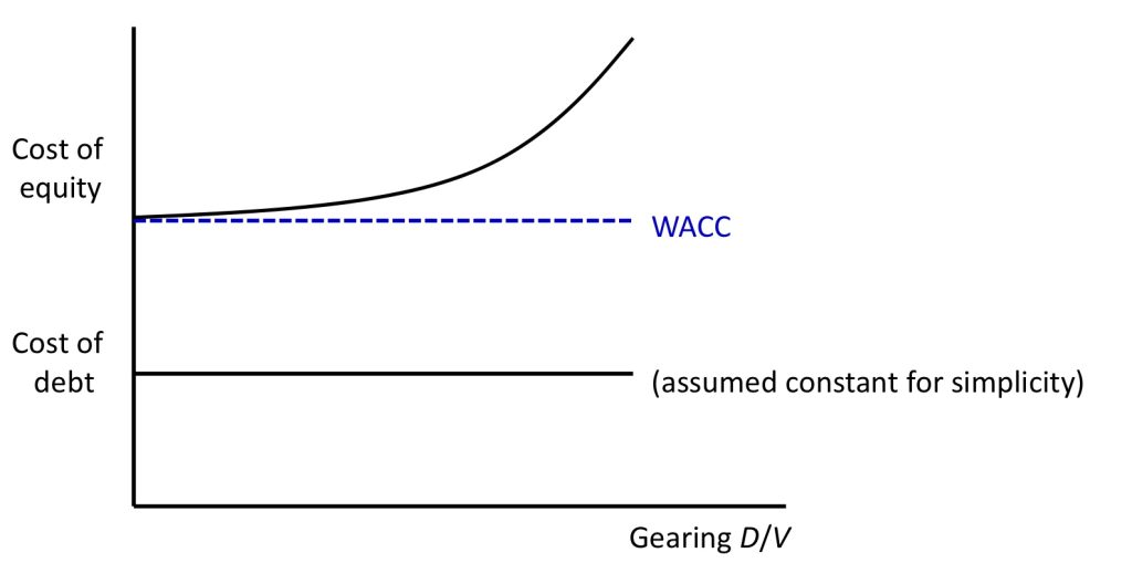
Since expected net cash flow (\(Y\)) and company value are the same for each company, the cost of equity for ungeared Co2 and WACC for geared Co1 must be equal. So WACC must be constant with respect to gearing.
Let the cost of equity for a company with no debt be \(R_{ungeared}\).
So we get a linear relation between cost of equity and D/E, assuming a constant cost of debt, assuming a constant cost of debt (and assuming \(R_{ungeared}>R_D\)). Implicly, changes in gearing structure (or how to finance the business) do not affect the WACC for a company.
The relation is shown in this figure
Violation of the constant debt assumption of course would make WACC unconstant.
MM Theory & Beta
In the CAPM, expected returns on assets differ because their betas differ.
, where \(\beta_{ungeared}\) denotes asset beta, and \( \beta_{geared}\) denotes actual beta of shares of a geared company (estimated from the market data).
A Modigliani-Miller Theorem for Open-Market Operations
Monetary policy determines the composition of the government’s portfolio. Fiscal policy (the size of the deficit on the current account) determines the path of net government indebtedness. Wallace showed that alternative paths of the government’s portfolio consistent with a single path of fiscal policy can be irrelevant. The irrelevance means that both the equilibrium consumption allocation and the path of the price level are independent of the path of the government’s portfolio.
Typos are there. See the original paper issued by Fed in 1979.
Reference
Modigliani, F. and Miller, M.H., 1958. The cost of capital, corporation finance and the theory of investment. The American economic review, 48(3), pp.261-297.
Wallace, N., 1981. A Modigliani-Miller theorem for open-market operations. The American Economic Review, 71(3), pp.267-274.
In statistics and control theory, Kalman filtering, also known as linear quadratic estimation (LQE), is an algorithm that uses a series of measurements observed over time, including statistical noise and other inaccuracies, and produces estimates of unknown variables that tend to be more accurate than those based on a single measurement alone, by estimating a joint probability distribution over the variables for each timeframe. The filter is named after Rudolf E. Kálmán, who was one of the primary developers of its theory.
Wikipedia
During my study in Cambridge, Professor Oliver Linton introduced the Kalman Filter in Time Series analysis, but I did not get it at that time. So, here is a revisit.
My Thinking of Kalman Filter
Kalman Filter is an algorithm that estimates optimal results from uncertain observation (e.g. Time Series Data. We know only the sample, but never know the true distribution of data or never know the true value when there are no errors).
Consider the case, I need to know my weight, but the bodyweight scale cannot give me the true value. How can I know my true weight?
Assume the bodyweight scale gives me error of 2, and my own estimate gives me error of 1. Or in another word, a weight scale is 1/3 accurate, and my own estimation is 2/3 accurate. Then, the optimal weight should be,
$$ Optimal Result = \frac{1}{3}\times Measurement + \frac{2}{3}\times Estimate $$
, where \( Measurement\) means the measurement value, and \(Estimate\) means the estimated value. We conduct the following transformation.
$$ Optimal Result = \frac{1}{3}\times Measurement +Esimate- \frac{1}{3}\times Estimate $$
Optimal Result = Esimate+\frac{1}{3}\times Measurement – \frac{1}{3}\times Estimate
Optimal Result = Esimate+\frac{1}{3}\times (Measurement – Estimate)
Therefore, we can get
Optimal Result = Esimate+\frac{p}{p+r}\times (Measurement – Estimate)
, where \(p\) is the estimation error and \(r\) is the measurement error.
For example, if the estimation error is zero, then the fraction is equal to zero. Thus, the optimal result is just the estimate.
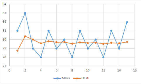
, where \(p_{n,n-1}\) is Uncertainty in Estimate, \(r_n\) is Uncertainty in Measurement, \(\hat{x}_{n,n}\) is the Optimal Estimate at \(n\), and \(z_n\) is the Measurement Value at \(n\).
The Optimal Estimate is updated by the estimate uncertainty through a Covariance Update Equation,
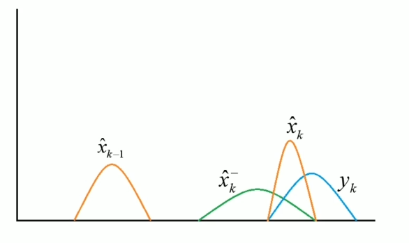
Intuitively, I need \( \hat{x}_{k-1}\) (, which is the weight last week) to calculate the optimal estimate weight this week \(\hat{x}_k\). Firstly, I estimate the weights this week \(\hat{x}_k^-\) and measure the weight this week \(y_k\). Then, combine them to get the optimal estimate weights this week.
Reading
The application of the Kalman Filter could be found in the following reading. Also, I will continue in my further study.