ARCH and GARCH
Let’s begin with the ARCH model.
ARCH Model
The ARCH model was initially raised by Engle (1982), and the ARCH model means the Autoregressive Conditional Heteroskedasticity model.
We assume here \(u_t\) is the return.
$$ u_t=\frac{P_t-P_{t-1}}{P_{t-1}} $$
$$u_t\sim N(0,\sigma_t^2)$$
The data-generating process (DGP) is like an AR form, as the name of ARCH. The volatility is autoregressively generated by \(u^2_i\).
$$\sigma_t^2=\delta_0+\sum_{i=1}^{p} \delta_i u_{t-i}^2$$
, where \(p\) is the number of lags, and \(\delta_i\) are a set of parameters. The DGP of that model shows that the volatility of the return is heteroscedastic, correlated with the squared term of the return per se.
For example, an ARCH(1) model is like,
$$ \sigma_t^2=\delta_0+\delta_1 u^2_{t-1} $$
- Stationarity
Note here we need our time series to be stationary for better forecasting. Thus, \(Var(u_t)=\sigma^2 \)
$$ Var(u_t)=\delta_0+\delta_1 Var(u_{t-1}) $$
$$ \sigma^2=\frac{\delta_0}{1-\delta_1} $$
As the variance has to be positive. We need \(\delta_0 > 0\), and \(\delta_1<1\).
- Estimation
For this time series data, OLS assumptions are violated, because our series are autoregressive heteroskedasticity.
Instead, the Maximum Likelihood Estimation (MLE) would be a better estimation method by assuming the probability distribution of variables.
MLE allows iterations to find parameters \(\delta\) that can maximise the maximum likelihood function.
GARCH Model
The ‘G’ in the GARCH model means ‘generalised’, and the GARCH model has a set of additional terms, \(\sum \gamma_i \sigma^2_i \). Thus, the DGP of the GARCH(p,q) model is as the following,
$$u_t\sim N(0,\sigma_t^2)$$
$$ \sigma_t^2=\delta_0 + \sum_{i=1}^{p} \delta_i u^2_{t-i} +\sum^q_{j=1} \gamma_j \sigma^2_{t-j} $$
ARMA-GARCH Model
That is a further application, in which the GARCH model is applied to mimic the movement of error terms in the ARMA model.
We initially assume an ARMA(p,q) model,
$$ y_t=\beta_0 +\sum^p_{i=1} \beta_i y_{t-i} + \sum^{q}_{j=1} \theta_j u_{t-j} +u_t$$
Then, we assume the error term here, \(u_t \sim GARCH(m,n)\).
$$ u_t \sim N(0,\sigma_t^2)$$
$$ \sigma_t^2 = \delta_0 +\sum^m_{i=1} \delta_i u_{t-i}^2 +\sum_{j=1}^n \gamma_n \sigma_{t-n}^2 $$
Reference
Engle, R.F., 1982. Autoregressive conditional heteroscedasticity with estimates of the variance of United Kingdom inflation. Econometrica: Journal of the econometric society, pp.987-1007.
近期经济观察
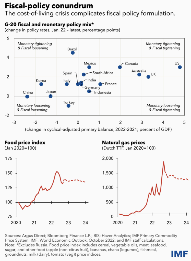
IMF Blog: Policymakers Need Steady Hand as Storm Clouds Gather Over Global Economy, by Pierre-Olivier Gourinchas, illustrated recent facts and economic data. Here is a brief presentation.
The world economic slowdown continues, Growth forecast in China is adjusted downward to 4.4% due to the weakening property sector and continued lockdowns by IMF.
Inflation
Rapidly rising prices, especially of food and the economy are causing serious hardship for households.
Inflation in China seems not that obvious, and the biggest problem, instead, is the slag of econ growth. Fortunately, wages are not increasing that much in most of the world economies. The hyperinflation raised from spikes in prices and wages is under control.
FOMC’s schedule of interest rate increases is expected to slow down, 50bp, in December.
The Chinese government is conducting loosening fiscal policy, stimulating the aggregate demand in part, and increasing the fiscal spending on infrastructure across countries through local financing platforms. The balance sheet is enlarging government leverage rate increases. The strong government is trying to raise confidence in individuals. However, monetary policy is limited due to the QT in the U.S. The exchange rate would be largely damaged if there were CB QE.
Energy Price
Food prices and energy prices surge to a high level and are expected to keep high as IMF expected.
OPEC decreases crude oil supply by 2 million barrer per day. IEA reported that US, as the target of global economic policy, released 15 million barrel of strategic crude oil reserve. US strategic crude oil reserve is about 401 million barrel.
OPEC和US对于石油价格博弈可能要追溯到2020年前,美国页岩油技术在2020年油价暴跌大背景下开始难以盈利。wait for further study.
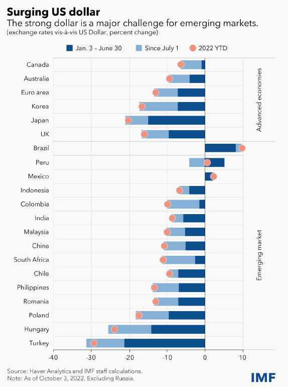
Strong USD
The strength of USD is a major challenge for many emerging market.
The appropriate response in most emerging and developing countries is to calibrate monetary policy to maintain price stability, while letting exchange rates adjust, conserving valuable foreign exchange reserves for when financial conditions really worsen.
In the tradeoff between the economic growth and the inflation, inflation seems become a piori target. The economy still has a bottom support, rigid demands such as foods, energy, accommodations etc. However, inflation is linked with the nomial term and could be even worsen off.
Why do Banks run?
Assumption
Entrepreneurs borrow from banks to invest in long-term projects. Banks themselves borrow from risk-averse households, who receive endowments every period. Households deposit their initial endowment in banks in return for demandable deposit claims. There is no uncertainty initially about the average quality of a bank’s projects in our model, so the bank’s asset side is not the source of the problem. However, there is uncertainty about household endowments (or equivalently, incomes) over time.
Process
Firstly, households deposit their initial endowments and have an unexpectedly high need to withdraw deposits.
Anticipated prosperity, as well as current adversity, can increase current household demand for consumption goods substantially.
As households withdraw deposits to satisfy consumption needs, banks will have to call in loans to long gestation projects in order to generate the resources to pay them. The real interest rate will rise to equate the household demand for consumption goods and the supply of these goods from terminated projects.
Results
Thus greater consumption demand will lead to higher real rates and more projects being terminated, as well as lower bank net worth. This last effect is because the bank’s loans pay off only in the long run, and thus fall in value as real interest rates rise, while the bank’s liabilities, that is demandable deposits, do not fall in value.
$$Asset = Liability + Equity$$
in the balance sheet, so as to banks. However, the difference is that banks’ assets are loans and liabilities are deposits from households. If the real interest rate increases, which conveys the increase in the discount rate, then the value of assets for banks would decrease (,by the present value of future cash flows). Liability (debts) keeps constant, then the equity of banks is destroyed.
Eventually, if rates rise enough, the bank may have negative net worth and experience runs, which are destructive of value because all manner of projects, including those viable at prevailing interest rates, are terminated.
Solution
How can this tendency towards banking sector fragility be mitigated?
- Capital Structure of Banks
One possibility is to alter the structure of banks. Long-term loans’ value is more volatile if the real interest rate fluctuates.
If banks financed themselves with long-term liabilities (in part我国政策行if the bank finances through long-term loans, that means A=D+E, `D is also volatile to the real interest rate changes, and moves in the similar direction as Asset) that fell in value as real interest rates rose, banks would be doubly stable. The bank hedge itself, hedging the assets by bank debts.
Deposits from households do not make banks stable, compared with financing through bank loans, because deposits could be withdrawn.
The authors stated that competition that banks strive for efficiency determines the capital structure of banks. I personally do not understand that idea, so I will leave it here.
P.S.
Diamond and Rajan (2001) 中指出,银行,作为金融中介,的功能是有human capital能量化或者保证depositors withdraw时 borrower能提供足够的liquidity还给lender (depositor)的问题。
- 2. Government Intervention
The government may have to intervene to pull the economy or consumption back into place. A typical way of doing so is through lower the interest rate.
The paper states that, reducing interest rates drastically when the financial sector is in trouble, but not raising them quickly as the sector recovers could create incentives for banks to seek out more illiquidity than good for the system. Such incentives may have to be offset by raising rates in normal times more than strictly warranted by macroeconomic conditions.
Put differently, reduce in interest rates could encourage banks to increase leverage or fund even more illiquid projects up front. This could make all parties worse off.
Reference
Diamond, D. and Rajan, R. (2009) (w15197) Illiquidity and Interest Rate Policy. Cambridge, MA: National Bureau of Economic Research DOI: 10.3386/w15197.
Diamond and Rajan’s Study about Financial Crisis 2008
The authors noted the financial crisis of 2008 was caused by mainly three reasons.
- U.S. financial sectors misallocated resources to real estate.
- Commercial and Investment banks had a large proportion of their instruments in their Balance Sheet.
- Investments were largely financed with short-term debts.
The following will illustrate why those facts happen.
1. Misallocation of Investment
Step 1. World Crisis pushed up risks.
The financial crisis in emerging markets, East Asia Econ Collapsed, `Russia Defaulted, South America, etc made investors circumspect.
Step 2. Capital Controls made CA surplus.
To react to those unexpected events and prevent domestic industries from the incumbents, governments started to conduct capital controls. Also, investors were unwilling to invest (they cut down investments and even consumptions) or charge a high-level risk premium. A number of countries became net exporters.
Step 3. “dot-com” bubble derived another global crisis.
Those exporters then had a current accounts surplus and transferred the CA surplus into “savings” (investment). Those savings were invested into the high-return business, the IT industry. However, another nightmare happened that is the “dot-com” bubble collapsed around the 2000s.
Step 4. CB QE and US financial innovations made a housing bubble
Central Banks QE, lowered the interest rate, which ignited demand for housing. The house price spiked. In the U.S., financial innovation (securitization) drew more marginal-credit-quality buyers into the market. The crisis manifested itself.
Step 5. Asymmetric information enforced the bubble.
Because rating agencies were at a distance from the homeowner, they could process only hard information. Asymmetric information enforced the bubble. Housing prices surged to prevent “default”.
Step 6. Securitization Iterate itself.
The slicing and dicing through repeated securitization of the original package of mortgages created very complicated securities. The problems in valuing these securities were not obvious when house prices were rising and defaults were few.
But as the house prices stopped rising and defaults started increasing, the valuation of these securities became very complicated.
2. Why Did Bank hold those instruments?
The key answer is bankers thought those securities were worthwhile investments, despite their risks. Risks were vague and unable to be evaluated.
it is very hard, especially in the case of new products, to tell whether a financial manager is generating true excess returns adjusting for risk, or whether the current returns are simply compensation for a risk that has not yet shown itself but that will eventually materialize.
Several facts manifested the problem.
- 1. Incentive at the Top
CEOs’ performance is evaluated based in part on the earnings they generate relative to their peers. Peer Pressure, which came from holding financial instruments to increase returns, mutually increased the willingness to hold those financial instruments.
- 2. Flawed Internal Compensation and Control
The top management wants to maximise the long-term bank value and goals. However, many compensation schemes are paid for short-term risk-adjusted performance. The divergency gave managers an incentive to take risks in the short term.
It is not said that the Risk management team is unaware of such incentives. However, they may be unable to fully control them, because tail risks, by the nature, are hard to quantify before they occur.
- 3. Short-term Debt
Given the complexity of bank risk-taking, and the potential breakdown in internal control processes, investors would have demanded a very high premium for financing the bank long term. By contrast, they would have been far more willing to hold short-term claims on the bank, since that would give them the option to exit — or get a higher premium — if the bank appeared to be getting into trouble.
In good times, short-term debt seems relatively cheap compared to long-term capital and the costs of illiquidity remote. Markets seem to favor a bank capital structure that is heavy on short-term leverage. In bad times, though, the costs of illiquidity seem to be more salient, while risk-averse (and burnt) bankers are unlikely to take on excessive risk. The markets then encourage a capital structure that is heavy on capital.
- 4. The Crisis Unfolds
Housing Price decreased, => MBS fall in value and becaome hard to price. Balance sheet destorted, and debt level held, and equity shrinked.
Every parties sold out, drived price down again and again.
Panic (no confidence) spreaded worldwide.
Interbank lendings were forzen as inadequate credits.
- 5. The `Credit Crunch
Banks were reluctant to lend due to two reasons. One possibility is that they worry about borrower credit risks. A second is that they may worry about having enough liquidity of their own, if their creditor demands funds.
- Dealing with the Crunch
Banks still fear threats from illiquidity. Illiquid assets still compose significant portions of banks and non-banl balance sheets. The price of those illiquid assets fluctuated largely, because liquidty asset could be easily exchanged or sold out for cash, but illiquid assets were unable to do so so that price shrinked and damaged the balance sheet. Debts held constant, but assets shrinked, resulting in shrinkage of equity, and increase in leverage and financial burden.
Coins have two sides. Low prices mean not only insolvent, but also tremendous buying opportunity. The pandic manified the expectation of insolvency, plus illiquid market condition made the fact that less money was availab to buy at the price. Selling iterated itself.
CB standed out, provided liquidty to financial institutes.
However, an interesting thing happened. CB’s intervention to lend against all manner of collateral may not be a unmitigated bless, because it may allow weak entities to continue holding illiquid assets.
Possible ways to reduce the overhand
1. Authorities offer to buy illiquid assets through auctions. `This can reverse a freeze in the market caused by distressed entities. Fair value from the aution can be higher than the prevailing market price. 2. government ensures the stability of financial system that holds illiquid assets through the recapitalization of entities that have a realistic possibility of survival. (我国,纳入国有).
Reference
Diamond, Douglas W. and Rajan, Raghuram G., The Credit Crisis: Conjectures About Causes and Remedies (February 2009). NBER Working Paper No. w14739, Available at SSRN: https://ssrn.com/abstract=1347262
A Great Introduction to the Nobel Prize Econ 2022
Here below is a great article introducing the Nobel Prize in Econ in 2022.
Later, I will start a series of studies about the journal articles from those Nobel Prize winners. Hopefully, that would help us understand the current crisis.
Reference
Bernanke, B., Gertler, M. and Gilchrist, S. The Financial Accelerator in a Quantitative Business Cycle Framework.
Diamond, D.W. and Dybvig, P.H. ‘Bank Runs, Deposit Insurance, and Liquidity’. JOURNAL OF POLITICAL ECONOMY, p. 19.
Unemployment Data in the U.S. Labour Market
The statistical data of unemployment rate released last week. 3.5% in September 2022, another lowest level even in history.
The U.S. economy is encountering still hgih level of inflation. To fight the inflation, one of the target of the Fed, the Federal Fund Rate has already been increase to about 3% to 3.25% in order to slow down the economy. However, the unemployment data shows the economy is seemingly continuously heating.
There several reasons explain the over-heated labour market.
- Individuals have already overcome the pandemic, and the consumption, especially service, are in high demands. There is even an overshooting of demands for labours.
- Many people leave the labour market, and are classified as distressed workers who are not included in the calculation of unemployment rate.
- Immigrant policy have changed since the Trump. To increase the employment rate for those “domestic” U.S. citizens, the immigrant policy has been not that friendly. Less low-cost labours inputed into the U.S. economy drives a gap of workers.
The low unemployment rate provides the Fed another inspiration of QT.
After QE
Why QE ?
By QE, the Fed increased the money supply to stimulate the aggregate demand in 2020 and 2021.
$$ Y=C+I+G+NX $$
By QE, more money were dumped into the economy. Two mainly used methods are (1) helicopter drops, and (2) banks/firms repo and CB reverse repo.
What happens after QE ?
- 1. Individuals got the more money in hands (mainly from Helicopter Drops in 2020) — Consumption increased. In the U.S., people who had SSN and were taxed a year before a certain time point were assured an opportunity of helicopter drops. Those money were highly likely ( and it really is) to transform to real demands in the market, because of the consumption habit in the U.S.
The Fed printed extra money and dumped into the economy. People spent those extra money to buy goods and service. Less Goods and Services were produced domestically in the U.S., while most of them were imported from Mexico, India, Russia, China, Mideast, etc. That is what I discussed before. The U.S. printed money (, which are worthless), and use “nothing” to reap goods and services from all over the world.
The above is one fact. Another is that there are still too much of money in the economy. Too much money chased too little goods. Like Milton Fridman said “Inflation is nothing but a monetary phenomenon”. There were no enough outputs (aggregate supply) to meet the increase in aggregate demand resulted from QE, then inflation surged.
- 2. Increase in supply of money dragged the interest rate down and thus reduced the financial cost for firms. Investment increased. This case is a bit different. In China, the CB conducted also QE to stimulate the economy especially in the current situation. However, the CB’s conduction is mainly through the Banking System. In this case, money are mainly poured into firms through loans not to individuals. Individuals are hardly able to get low-cost money because on the one hand them may not have enough pledges, and on the other hand people are fear to invest in the real estate, coz the real estate bubbles are in the edge of collapse although the gov is trying to keep the mkt stable.
Pros and Cons are there. Advantages are (1) firms that got the low-cost money are most likely state owned firms. In this case, there are “relative high probability” of safety. (2) firms encounter low financial cost and could have direct impact on infrastructures. Disadvantages are also that (1) money could not be directly given to individuals, no real happiness or utility increase for those family. Family based businesses are still suffering the plunges in demands and undergo bankruptcy. (2) too much money chase too little high-quality assets that can have potential positive expected return or payoffs. Money circulates in the economy, and costs circulates as well to increase. On the one hand there is low efficiency, on the other hand extra money does not contribute to stimulate the economy. Financial System discoodinates.
Differential Equation
Statistics
The notes are not only a review for the preparation of quants but also hopefully a learning note for my babe.
Key Points
1. Preliminaries
Firstly and most importantly, I need to declare what is statistics and why shall we learn statistics. The following is only based on my own understanding. My understanding is pretty limited (I got only a master’s degree, so I am definitely not an expert in Statistics) and subjective, please provide your suggestions and even your blames to me. Glad to know your ideas.
1.1 What is Statistics?
From my understanding, Statistics is a tool, characterized by mathematics, to explain the world. Such a bull shit am I talking.
Be serious. I may say that statistics is a process to estimate the population by samples.
To do a study about the population is always costly, and pretty much unpredictable. For example, to do tests in the individual level, we have to collect data from all the people. The population census could only be done in a national level and conducted by the gov. Even so, the census is unable to be performed in a year-by-year basis, and there are measurement errors always. Thus, a more cost-effective way would be to estimate the population through the data from a small set of people who are randomly selected.
Another example could be the weather forecast, which is similar to doing a time series analysis or panel data analysis. The forecast may most likely be biased because things change unpredictably and irregularly. So we may say that is even impossible to and the full data to estimate the population (factors related to weather in this case). Thus, a simpler way might be that we collect different factors and historical data such as temperature, because we may assume the temperature changes are consistent over a short period of time.
However, there are gaps between population and sample. How could we connect those gaps? The answer is Statistics. Statistics provide some mathematical proven methods to make the sample have a better capture of the population, based on assumptions.
Let’s begin our study.
2. Probability
2.1 Conditional Probability
$$
P(A|B)=\frac{P(A\cap B)}{P(B)}\\ \\ P(A\cap B)=P(A|B)\times P(B)
$$
2.2 Mutually Exclusive and Independent Events
$$
P(A\cap B)=0 \\ \\ P(A\cup B)=P(A)+P(B)
$$
If two events are independent, then
$$
P(A|B)=P(A) \\ \\ so, \quad P(A\cap B)=P(A)\times P(B)
$$
3. Random Variables – r.v.
3.1 Definition
Random Variables: X, Y, Z
Observations: x,y,z
3.2 Probability Mass/Density Funciton – p.d.f. (For Discrete r.v. or Continuous r.v.)
3.2.1 Definition
p.d.f captures the probability that a r.v. X has a given value of x.
$$
P(X=x)=P(x)
$$
3.2.2 Properties of p.d.f.
- \(f(x)\geq 0\), since probability is always positive.
- \(\int_{-\infty}^{+\infty} f(x)\ dx=1\)
- \(P(a<X<b)=\int_a^b f(x) \ dx\)
Replace the integral with summation for discrete r.v.
P.S. For continuous r.v. X, P(X=x)=0. That means for a continuous r.v., any points on the p.d.f have a zero probability.
For example, the probability of selecting a number “3” among 1 to 10 is zero.
3.3 Cumulative Distribution Function – c.d.f
$$
F(X)=P(X\leq x) \\ \\ f(x)=\frac{d}{dx} F(x)
$$
3.4 Expectation
$$
E(X)=\mu \\ \\ E(X)=\int_{dominX}x\cdot f(x)\ dx=\sum_x x\cdot P(X=x) \\
$$
3.5 Variance and Standard Deviation
$$
Var(X)=\sigma^2\\ \\ Var(X)=E(X-E(X))=E(X^2)-(E(X))^2 \\ =\frac{\sum (x-\mu)^2}{n}=\frac{\sum x^2}{n}-\mu^2
$$
3.6 Moments
The first moment, \(E(X)=\mu\).
The n^{th} moment, \(E(X^n)=\int_x x^n\ f(x)\ dx\).
The second central moment is about mean. \(E(X-E(X))=\sigma^2\), Variance.
The third central moment, \(E(X-E(X))^3. Skewness = \frac{E(X-E(X))^3}{\sigma^3}\). Standard normal dist has a Skewness of 0. (Right or Left Tails)
The Fourth central moment, \(E(X-E(X))^4. Kurtosis = \frac{E(X-E(X))^4}{\sigma^4}\). Standard normal dist has a Kurtosis of 3. (Fat or This, Tall or Short).
3.7 Covariance
$$
Cov(X,Y)=E[(X-E(X))(Y-E((Y))]\\ =E(XY)-E(X)E(Y)
$$
4. Distribution
The meaning of distributions, and the properties (mean & var).
4.1 Bernoulli DIst
4.2 Binomial Dist
4.3 Possion Dist
$$
X \sim Possion(\lambda)\\ \\p.d.f \quad P(X=x)=\frac{e^{-\lambda}\lambda^x}{x!}\\ E(X)=\lambda,\quad Var(X)=\lambda
$$
4.4 Normal Dist & Standard Normal
$$
X\sim N(\mu,\sigma^2)\\ \\ p.d.f. \quad f(x)=\frac{1}{\sqrt{2\pi \sigma^2}}exp\frac{(x-\mu)^2}{2\sigma^2}
$$
For a standard normal dist,
$$
X\sim N(0,1)\\ \\ E(X)=0,\quad Var(X)=1
$$
4.4.1 Standardisation
$$
Z=\frac{X-\mu}{\sigma}
$$
4.4.2 Properties of Normal Dist
One / Two /Three standard deviation regions.
5. Central Limit Theorem – CLM
i.i.d. – independent identical distributed
Suppose X_1,X_2,…,X_n are n independent r.v., each has the same distribution, and as the number n increases, the distribtuion of
$$
X_1+X_2+…+X_n\\\\ \text{and,}\\\\ \frac{X_1+X_2+…+X_n}{n}
$$
would behave like a normal distribution.
Key facts:
- The distribution of X is not stated. We do not have to restrict the distribution of r.v.s, as long as they are in the same dist.
- If X is a r.v. with mean \(\mu\) and standard deviation \(\sigma\) from a random dist, the CLT tells that the distribution of the sample mean, \(\bar{X}\) is normal dist.
$$
E(\bar{X})=E(\frac{\sum X}{n})=\frac{\sum E(X)}{n}\\=\frac{n\mu}{n}=\mu\\ \\ $$
$$Var(\bar{X})=Var(\frac{\sum X}{n})=\frac{\sum Var(X)}{n^2}\\=\frac{n\sigma^2}{n^2}=\frac{\sigma^2}{n}\\
$$
Therefore, we would get the distribution of \bar{X},
$$
\bar{X}\sim N(\mu,\frac{\sigma^2}{n})
$$
By standardising it,
$$
\frac{\bar{X}-\mu}{\frac{\sigma}{\sqrt{n}}}\sim N(0,1)
$$
Also, for S_n=X_1+X_2+…+X_n.
$$
S_n \sim N(n\mu,n\sigma^2)\\\\ \frac{S_n-n\mu}{\sqrt{n}\sigma}
$$
The more observations there are, the more similar the distribution to normal would be. Also, a less standard deviation means the estimate has fewer variations and is more accurate.
Why is CLT important?
It is important because it provides a way to use repeated observations to estimate the whole population, which is impossible to be observed.
6. A Few Notations
Recall, our aim of using statistics is to find the true population. We may assume the true population follows a distribution, and that distribution has some parameters. What we are doing right now is to use the sample data (feasibly collectible) to presume the population parameters.
- Estimator: a function, using sample or available data, to estimate the population. i.e. \(\bar{x}\) and \(S^2\).
- Estimate: the value/figure we truly calculated. By inputting data into the estimator, the output is the estimate.
Population (Population Parameters that we want to get but can never get)
Population Mean: \(\mu=\frac{\sum x_i}{N}\).
Population Variance: \(\sigma^2=\frac{\sum (x_i-\mu)^2}{N}\).
Sample Estimator
Sample Mean: \(\bar{x}=\frac{\sum x_i}{N}\).
Sample Variance: \(\hat{\sigma}^2=\frac{\sum (x_i-\bar{x})^2}{N}\).
Throw data into sample estimators would get the estimates, and those estimates are then applied to presume the population parameters.
Remember that sample is only part of the population, we collect data from the sample because they are more accessible and feasible to get. Still, we need to use our sample data to be representative of the population, or in another word, to have some foreseers about the whole population. Therefore, we use a different notation for sample statistics.
An important aspect is that we need our sample to have better representativeness of the population. There are some measurements.
6.1 Unbiasedness
If \(E(\bar{X})=\mu, \text{or} \ E(S^2)=\sigma^2 \)(the expectation of our sample estimate is equal to the population), then we would say the estimator is unbiased.
The unbiased estimator of sample variance is \(S^2=\frac{\sum (x_i-\bar{x})^2}{n-1}\).
$$
E(S^2)=\sigma^2
$$
Why the denominator is “n-1”?
There would be a long discussion to talk about that. We can simply understand “-1” as the adjustment of the \(\bar{x}\) in the numerator because \(\bar{x}\) is calculated to represent the population mean \(\mu\) and \(\bar{x}\) is not intrinsically available (it is costly, to save for the cost, the denominator has a deduction).
In sum, \(S^2\) is an unbiased estimator of population variance, \(\sigma^2\). We also have a special name for the sample standard deviation, Standard Error, s.e..
6.2 Consistency
If there is an estimator such that as \(n\rightarrow \infty\) , the estimator goes close to the population parameter, we may say that estimator is consistent.
For example, although \(\hat{\sigma}^2=\frac{\sum (x_i-\mu)^2}{N}\) is biased, it is consistent if the number of observation keeps increasing.
Flaws of discussion is available in this section, awaiting to be updated.
7. Estimation
7.1 Maximum Likelihood Estimation – MLE
By assuming a probability distribution of the r.v. X, fitting into sample observations and trying to find the parameters that can maximise the joint probability (likelihood function).
To illustrate the problem, we need to find the parameters \lambda that can maximise the likelihood function.
$$
\lambda_0=\text{arg}\max_{\lambda}\ L(\lambda;x)
$$
The value of the parameters \(\lambda_0\) is our MLE estimator. (Remember what estimator is? See section 6).
For example
Assume r.v. \(X\sim N(\mu,\sigma^2)\). Let \(x_1,x_2,…,x_n\) be a random sample of i.i.d. observations. We use MLE to find the value of \(\mu\) and \(\sigma^2\). So, we need to maximise the log-likelihood function (instead of using the likelihood function, we do a logarithm transformation for easier calculation. Because the log transformation is monotonic, the transformation is legal).
$$
\begin{align*} f(x_1,x_2,…,x_n;\mu,\sigma^2)&=f(x_1,\mu,\sigma^2)f(x_2,\mu,\sigma^2)…f(x_n,\mu,\sigma^2)\\ \text{Let}\\L(\mu,\sigma^2;x_1,x_2,…,x_n)&=log \ l(\mu,\sigma^2;x_1,x_2,…,x_n)\\ &=log\ f(x_1;\mu,\sigma^2)+log\ f(x_2;\mu,\sigma^2)+…+log\ f(x_n;\mu,\sigma^2)\\ &=\sum_{i=1}^N log\ f(x_i;\mu,\sigma^2) \\ \text{Plug in }f(x;\mu,\sigma^2)=\frac{1}{\sqrt{2\pi \sigma^2}}exp\frac{(x-\mu)^2}{2\sigma^2} \\ L(\mu,\sigma^2;x_1,…,x_n)&=log\ [\sum \frac{1}{\sqrt{2\pi \sigma^2}}exp\frac{(x-\mu)^2}{2\sigma^2} ] \\ &=-\frac{n}{2}log\ (2\pi)-n\cdot log\ (\sigma)-\frac{1}{2\sigma^2}\sum (x_i-\mu)^2 \end{align*}
$$
F.O.C.
$$
\hat{\mu}_{MLE}=\frac{1}{n}\sum x_i \\ \hat{\sigma^2}_{MLE}=\frac{1}{n}\sum (x_i-\mu)^2
$$
We would find the MLE estimators are the same as the OLS estimator in the following section.
7.2 Regression
Assume a linear model through which we can have a minimum sum mean squared.
$$
\hat{\beta}_{all}=arg\min_{\beta_{all}}\sum(y_i-\hat{y_i})^2\\ \Leftrightarrow\\ \hat{\beta}=arg\min_{\beta}(Y-\hat{Y})'(Y-\hat{Y})\\ \\
$$
, where
$$
\hat{y}=\hat{\beta_0}+\hat{\beta_1}x_1+…+\hat{\beta_k}\\ or,\quad \hat{Y}=X\hat{\beta}
$$
F.O.C.
$$\hat{\beta}=(X’X)^{-1}X’Y$$