The Arrow-Pratt coefficient of absolute risk aversion
Definition (Arrow-Pratt coefficient of absolute risk aversion). Given a twice differentiable Bernoullio utility function \(u(\cdot)\),
$$ A_u(x):=-\frac{u”(x)}{u'(x)} $$
Risk-aversion is related to concavity of \(u(\cdot)\); a “more concave” function has a smaller (more negative) second derivative hence a larger \(u”(x)\).
Normalisation by \(u'(x)\) takes care of the fact that \(au(\cdot)+b\) represents the same preferences as \(u(\cdot)\).
In probability premium
Consider a risk-averse consumer:
1. prefers \(x\) for certain to a 50-50 gamble between \(x+\epsilon\) and \(x-\epsilon\).
2. If we want to convince the agent to take the gamble, it could not be 50-50 – we need to make the \(x+\epsilon\) payout more likely.
3. Consider the gamble G such that the agent is indifferent between G and receiving x for certain, where
$$G= \begin{cases} x+\epsilon, & \text{with probability $\frac{1}{2}+\pi$}.\\ x-\epsilon, & \text{with probability $\frac{1}{2}-\pi$ } \end{cases}$$
4. It turns out that \(A_u(x)\) is proportional to \(\pi/\epsilon\) as \(\epsilon \rightarrow 0\); i.e., \(A_u(x)\) tells us the “premium” measured in probability that the decision-maker demands per unit of spread \(\epsilon\).
ARA.
Decreasing Absolute Risk Aversion. The Bernoulli function \(u\cdot)\) has decreasing absolute risk aversion iff \(A_u(\cdot)\) is a decreasing function of \(x\). Increasing Absolute Risk Aversion… Constant Absolute Risk Aversion – Bernoulli utility function has constant absolute risk aversion iff \(A_u(\cdot)\) is a constant function of \(x\).
Relative Risk Aversion
Definition (coefficient of relative risk aversion). Given a twice differentiable Bernoulli utility function \(u(\cdot)\),
$$ R_u(x):=-x\frac{u”(x)}{u'(x)}=xA_u(x) $$
There could be decreasing/increasing/constant relative risk aversion as above.
Implication: DARA means that if I take a 10 gamble when poor, I will take a10 gamble when risk. DRRA means that if I gamble 10% of my wealth when poor, I will gamble 10% when rich.
Ramsey (1928), followed much later by Cass (1965) and Koopmans (1965), formulated the canonical model of optimal growth for an economy with exogenous ‘labour augmenting technological progress. The R.C.K model (or called. Ramsey (Neo-classical model) can be considered as an extension of the Solow model but without an assumption of a constant exogenous saving rate.
Assumptions
Firms
Identical Firms.
Markets, factors markets and outputs markets, are competitive.
Profits distributed to households.
Production fucntion with labour augmented techonological progress, \(Y=F(K,AL)\). (Three properties of the production: 1. CRTS; 2. Diminishing Outputs, second derivative<0; 3. Inada Condition.)
\(A\) is same as in Solow model, \(\frac{\dot{A}}{A}=g\). Techonology grows at an exogenous rate “g”.
Households
Identical households.
Number of households grows at “n”.
Households supply labour, supply capital (borrowed by firms).
The initial capital holdings is \(\frac{K(0)}{H}\)., where \(K(0)\) is the initial capital, and \(H\) is the initial number of households.
Assume no depreciation of capital.
Households maximise their lifetime utility.
The utility fucntion is constant-relative-risk-aversion (CRRA).
The lifetime utility for a certain household is represented by,
We denote \(w(t)=W(t)/A(t)\) as the efficient wage rate, then we get,
$$ w(t)=f(k(t))-k(t)f'(k(t)) $$
Another key assumption of this model is,
$$ \dot{k}(t)=f(k(t))-c(t)-(n+g)k(t) $$
, which represents the actual investment (outputs minus consumptions), \(f(k(t))-c(t)\); and break-even investment, \((n+g)k(t)\). The implication is that population growth and technology progress would dilute the capital per efficient work.
The difference with the Solow model is that we do not assume constant saving rate “s” in \(sf(k)\) now, instead we assume the investment as \(f(k)-c\).
Households
The budget constraint of households is that: the PV of lifetime consumption cannot exceed the initial wealth and the lifetime labour incomes.
, where \(R(t):=\int_{\tau=0}^ t r(\tau) d\tau\) to represent the discount rate overtime. When \(r\) is a constant, \(R(t)=r\cdot t\) and \(A(t)=A(0)e^{rt}=A(0)e^{R(t)}\).
We plug the \( \begin{cases} C(t)=A(t)c(t)\\L(t)=L(0)e^{nt}\\A(t)=A(0)e^{gt} \end{cases} \) into households’ lifetime utility function (objective function), and then get the,
, where \(B:=A(0)^{1-\theta} \frac{L(0)}{H}\) and \(\beta:=\rho-n-(1-\theta)g\) (we need \(\beta>0\) to make the utility function convergence), and the utility function is, \(u(c_t)=\frac{c_t^{1-\theta}}{1-\theta}\).
The budget constraint is the households’ lifetime budget constraints divided by \(A(0)\) and \(L(0)\),
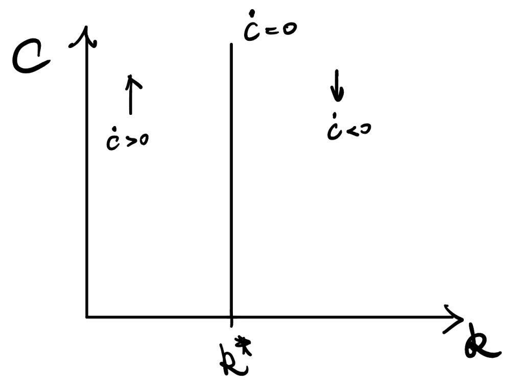
Therefore, we find the time-path of consumption depends on \(f'(k)\). We define \(k*\) is the solution when \(f'(k)=\rho+\theta g\). So, at \(k^*\), the numerator of RHS equals zero.
As \(f(k)\) is an increasing function but with diminishing returns, so \(f”(k)<0\) and that means \(f'(k)\) is a decreasing function in k. Thus,
at \(k<k^*\), \(f(k)>\rho+\theta g\) and \( \frac{\dot{c_t}}{c_t} >0\);
at \(k>k^*\), \(f(k)<\rho+\theta g\) and \( \frac{\dot{c_t}}{c_t} <0\).
Figure 1
The dynamics of k
We recall the assumption,
$$ \dot{k}(t)=f(k(t))-c(t)-(n+g)k(t) $$
At \(\dot{k}=0\), consumption, \(c(t)=f(k(t))-(n+g)k(t)\), equals outputs minus break-even investment.
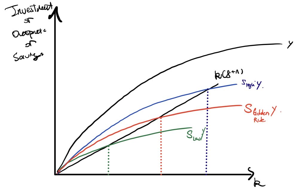
We now consider the Solow model without the depreciation term. Recall the difference between the RCK model and the Solow model is that we do not assume a constant saving rate over time, but other things keep similar. Thus, the term \(c(t)\) is “equivalent” to \(sy\) in Solow model.
Figure 2
In the Solow model, changes in saving rate would change the magnitude of \(sy\) curve. The Golden Rule saving rate is “s” that maximises consumption (the difference between Y and the interaction between \(sy\) and \(k(g+n)\)). The shape of the production function determines the property of the Golden Rule saving rate.
An equilibrium level of consumption is determined in mainly two steps. 1. the interaction between saving \(sy\) and \((n+g)k\) determines the \(k^*\). 2. plug \(k^*\) back to \(sy\) and find the difference between outputs and savings to get consumption.
We here focus on the second step, the equilibrium level of \(k^*\) determines consumption and thus consumption is a function of \(k^*\). At a lower saving rate (see Figure 2), \(k^*\) is too small, so there is less consumption. At a higher saving rate, \(k^*\) is too large, so there is also less consumption. Therefore, we can find that consumption is in a quadratic form w.r.t. \(k^*\).
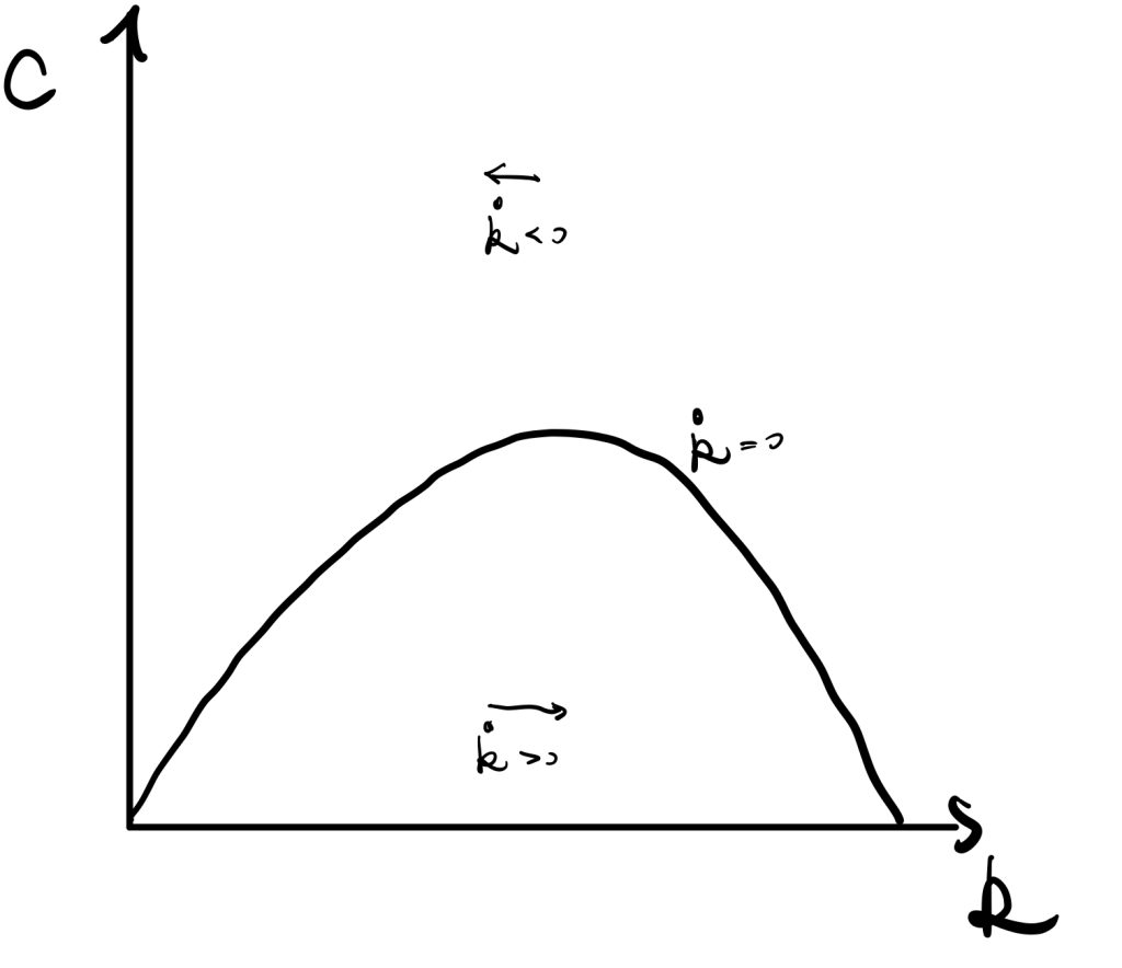
Figure 3. \(c(t)=f(k(t))-(n+g)k(t),\ \dot{k}=0\)
$$ (s\downarrow) \Leftrightarrow k \downarrow \to c \downarrow$$
$$ (s\uparrow) \Leftrightarrow k \uparrow \to c \downarrow$$
Or, we can consider consumption as the difference between \(y\) and \((n+g)k\). The wedge like area gets large and then shrinks.
Overall, the above facts make the \(\dot{k}=0\) curve.
Recall \( \dot{k}(t)=f(k(t))-c(t)-(n+g)k(t) \).
Above the curve where \(c\) is large, then \(\dot{k}<0\) so \(k\) decreases. Below the curve where \(c\) is small, then \(\dot{k}>0\) so \(k\) increases. Implication is that if less consumption, then more saving, \(\dot{k}\) increases.
Phase Diagram.
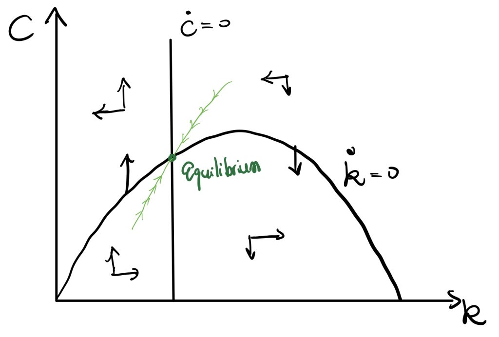
Figure 4
Combining Figure 1 and Figure 3, we get the above Phase Diagram. The equilibrium is shown in the figure above.
P.S. We can prove that the equilibrium is less than Golden Rule level \(k^*_{GoldenRule}\) (which is the maximum point in the quadratic shaped curve). The proof is the following,
The value of k at \(\dot{c}=0\) is \(f'(k)-\rho-\theta g=0\), and the Golden Rule level is \(c=f(k)-(n+g)k\) (as we illustrated before), and take f.o.c. w.r.t. k to solve the Golden rule k. \(\frac{\partial c}{\partial k}=0 \to f'(k)=n+g\). Therefore, we get,
$$ \begin{cases} f_1:=f'(k_{equilibrium})=\rho+\theta g \quad\text{equilibrium in phase diagram}\\ f_2:=f'(k_{GoldenRule})=n+g\quad\text{golden rule level}\end{cases}$$
$$ \rho+\theta g>n+g \quad \text{by our assumption of \beta convergence}$$
So, we get,
$$ f_1>f_2 $$
$$ k_{equilibrium}< k_{GoldenRule} $$
Thus, we find the equilibrium level capital per efficient workers, \(k_{equilibrium}\), must be less than the Golden Rule level \( k_{GoldenRule} \).
From the phase diagram, we can get the saddle path that can achieve equilibrium.
BGP
At the Balanced Growth Path, the economy is in equilibrium. So the time-paths satisfy \( \frac{\dot{c}}{c}=0, and \frac{\dot{k}}{k}=0 \). Therefore, we can get the BGP of others,
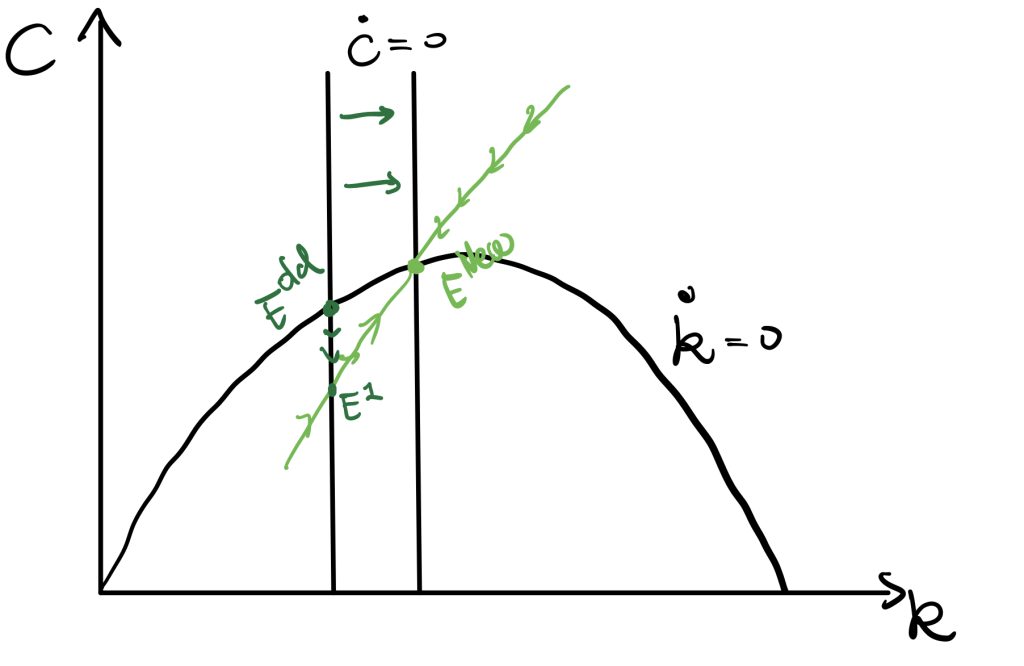
Assumption: government conducts government purchases, \(G(t)\). The government purchases do not affect the utility of private sectors, and future outputs. Government finances, G(t), by lump-sum taxes.
We can consider the crowding-out effect. Under full employment, government purchases take away part of the consumptions. In our case, government spending takes away some of the savings. Therefore, the dynamics of capital per efficient workers become (the minus government spending term shifts the curve downward by G(t)),
$$\dot{k}(t)=f(k(t))-c(t)-G(t)-(n+g)k(t)$$
In short, government purchases would make the economy achieve a new equilibrium where there is less consumption but the same capital (investment from the private sector) level. Also, the saddle path moves downward.
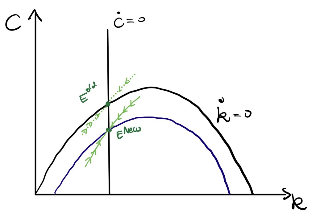
\(\rho\) Changes
A fall in \(\rho\) can be considered as the effect of monetary policy. A fall in \(\rho\) would result in a movement of \(\dot{c}=0\) curve to the right by the equality, \(\frac{\dot{c}}{c}= \frac{r(t)-\rho-\theta g}{\theta} =\frac{f'(k)-\rho-\theta g}{\theta}\).
P.S. \(\dot{c}=0 \Leftrightarrow f'(k)=\rho-\theta g \to k=f’^{-1}( \rho-\theta g )\)
As \(\rho\) changes, a new path generates. The economy is at \(E^1\), and then follows the new path moving to \(E^{new}\). We would finally end up with a new equilibrium with higher consumption.
We replace this non-linear equation with the linear approximation, so we take the first order Taylor approximation around the equilibrium \(k^*\) and \(c^*\).
We then replace \( \dot{c}=\frac{f'(k)-\rho-\theta g}{\theta}c \) ) and \( \dot{k}=f(k(t))-c(t)-(n+g)k(t) \) into \( \dot{k}_{approx} \) and \( \dot{c}_{approx} \). Also, we denote \(\tilde{c}=c-c^*\) and \(\tilde{k}=k-k^*\).
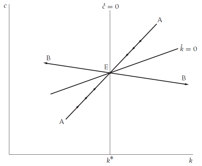
From the above two equations we can find growth rate of \(\dot{\tilde{c}}_{approx}\) and \( \dot{\tilde{k}}_{approx} \) depend only on the ratio, \(\frac{\tilde{k}}{\tilde{c}}\).
Later, we apply a very strong assumption that \(\tilde{c}\) and \(\tilde{k}\) changes at the same rate, and also the rate make LHS of two equations equal. By this assumption, we denote,
We can see \(\mu\) must be negative, otherwise the economy cannot converge (see the path BB). If \(\mu<0\), the economy would be in the path AA instead. The path is the saddle path of R.C.K. model.
Applying such as the Cobb-Douglas form production, we can plug second derivatives of the production into \(\mu\) and get the speed of adjustment.
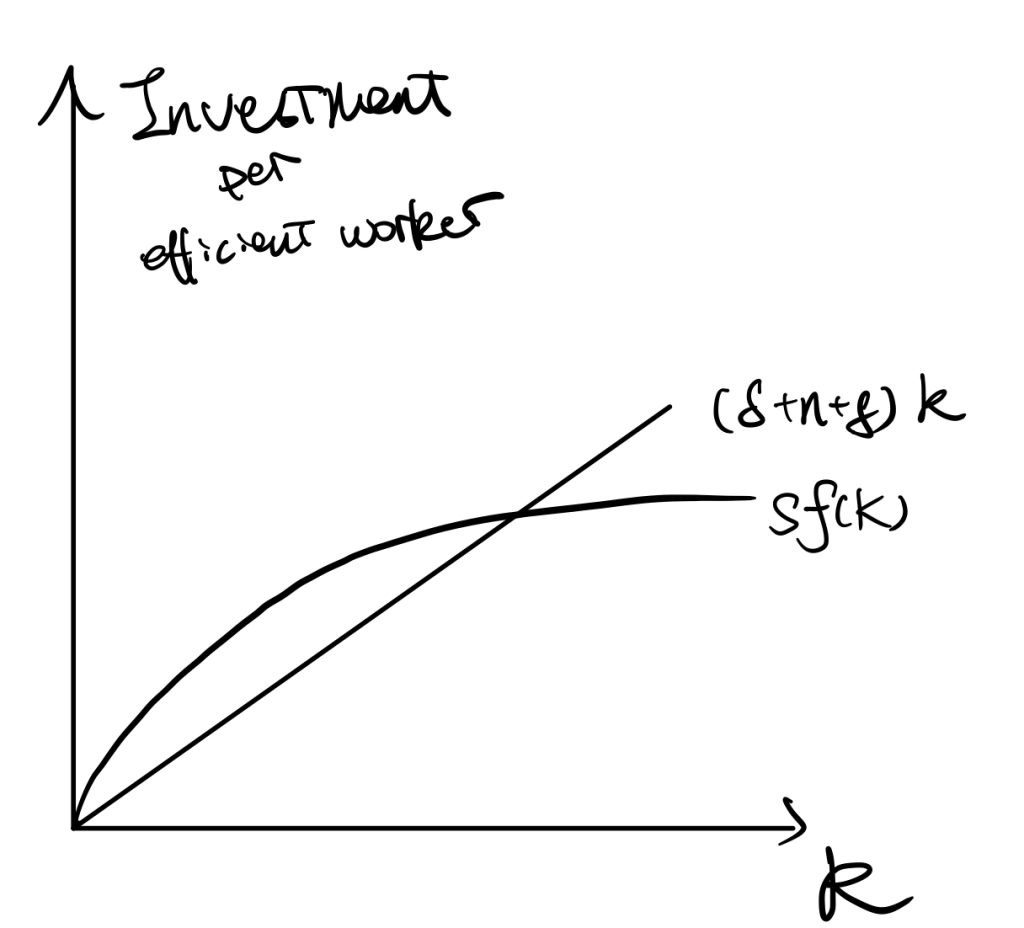
The current mostly used Solow model always have a depreciation term, and thus the law of motion becomes, \(\dot{K}=I-\delta K\).
The mainstream model has different assumptions about the production function as well. For example, technological progress is generally added. 1. \(Y=AF(K,L)\) in which technology is exogenous, and it could be called Hicks-neutral; 2. \(Y=F(K,AL)\) that can represent the efficient workers, labour-augmented, or Harrow-neutral; 3. \(Y=F(AK,L)\) in which the technological progress is capital augmented.
Applying for example the labour-augmented technology and \( \frac{\dot{A}}{A}=g\) , we can simply solve the Solow model as the following,
, where \(y=\frac{Y}{AL}\) and \(\frac{K}{AL}\) represent the output/capital per efficient works. Therefore, if \(\dot{k}=0\), then \(sy=(\delta+g+n)k\).
The stable point of k is \(k^*\) in which \(sf(k)=(\delta+n+g)k\).
We always the Cobb-Douglas function to represent the production function, because it satisfies CRTS, increasing and diminishing assumptions, and the Inada conditions (\(\lim_{k\rightarrow0}f'(k)=\infty; \lim_{k\rightarrow \infty}f'(k)=0\), Inada, 1963 ).
In the following, we would all analyse the model using efficient works to do analysis.
Balance Growth Path
All the following is assuming the economy is at the steady state or stable point.
For \( \frac{\dot{K}}{K} \),
$$ k=\frac{K}{AL} $$
By taking logritham,
$$ ln(k)=ln(K)-ln(A)-ln(L) $$
By taking differentiation and set \(\dot{k}=0\) (based on our previous derivations of finding the steady state condition).
In summary, the BGP is a situation in which each variable of the model is growing at a constant rate. On the balanced growth path, the growth rate of output per worker is determined solely by the rate of growth of technology.
P.S. Technology Independent of Labour And Capital
Applying for example the Type 1 case and \( \frac{\dot{A}}{A}=g\) , we can simply solve the Solow model as the following,
We would not use capital per efficient worker here, because labour is not technology-augmented by assumption. Instead, we simply assume capital per capita, \(k=\frac{K}{L}\). We can easily get the relationship,
We expand output per se (demoninator) by Euler’s Theorem \(Y=AF’_1K+AF’_2L\) (A is now outside the production function), and then calculate the percentage changes of outputs,
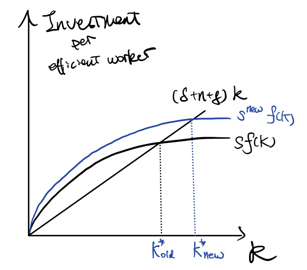
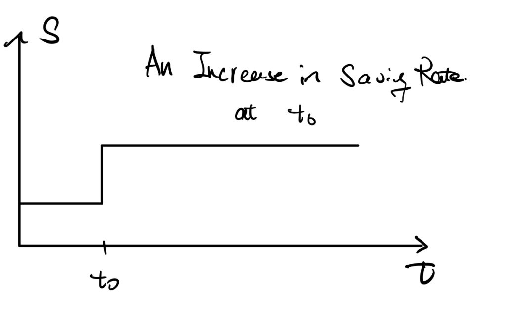
We now consider first how does changes in the saving rate affect those factors.
The determinants of saving rate are, for example, uncertainty or decrease in expected income, and required pension rate.
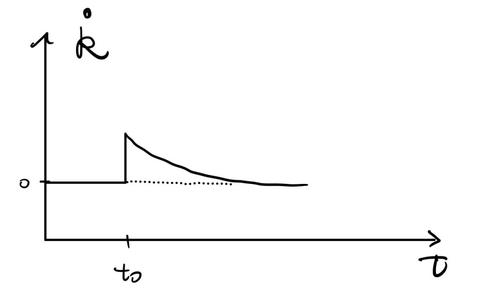
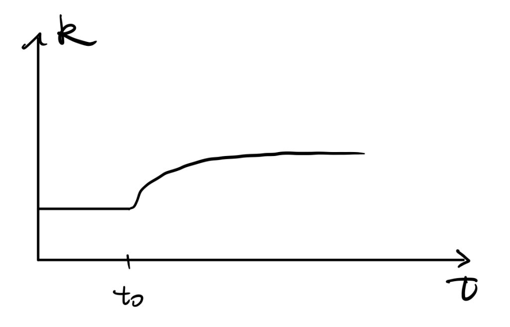
See the following figures,
An increase in the saving rate would result in an increase in the investment curve. \(\dot{K}=I-\delta K\) tells that there would be a huge increase in \(\dot{K}\) initially, and by the shape of production function, the difference diminishes until achieving the new stable point \(k^*_{new}\).
As \(\dot{k}\) is a derivative of \(k\) w.r.t. \(t\), we can easily get the time path of \(k\) as the following,
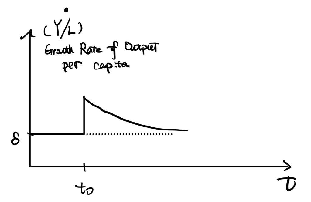
Another important factor is the growth rate of output per capita,
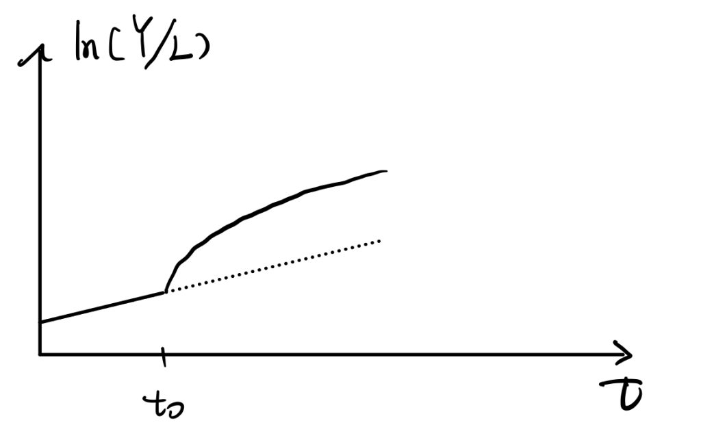
Also \(ln(Y/L)\),
For this one, we can prove that the slope of \(ln(Y/L)\) is \(\dot{ln(Y/L)}=\frac{\partial}{\partial t}[ln(Y)-ln(L)]=(g+n)-n=g\), so it grows constantly at rate “g” before \(t_0\). Later growth rate of Y jumps makes the slope of \(ln(Y/L)\) increases, but \(ln(Y/L)=g\) when achieves a new steady state and \(ln(Y/L)\) keeps growing at “g” in the long run.
The Speed of Convergence
Way 1
We follow our Solow model with labour-augmented technology. The time path of changes of capital per efficient works is,
$$ \dot{k}=sy-(\delta+n+g)k$$
$$ \dot{k}=sy-(\delta+n+g)k$$
At the steady state, \(\dot{k}=0\), so \( sy-(\delta+n+g)k \). We then plug in the Cobb-Doglas production function and denote \(y=\frac{Y}{AL}=\frac{K^{\alpha}(AL)^{1-\alpha}}{AL}=k^{\alpha}\), we can find the \(k^*\),
To find the speed of convergence, we would focus on the time path of k around \(k^*\). Or approximate the time-path by taking first-order Taylor expansionaround \(k^*\) to approximate,
$$ G(k)\approx G(k^*)+G'(k^*)(k-k^*) $$
As \(G(k^*)=0\) by our proof of steady state condition, thus,
Therefore, we find the mathematic expression of the convergence speed, \( (1-\alpha)(\delta+g+n) \). It is the measure of how quickly k changes when k diviates from \(k^*\). Also, we find that the growth rate \( G(k)=\frac{\dot{k}}{k} \) depends on both the convergence speed and \( \frac{k-k^*}{k^*} \), which is how far k deviates from its steady state level.
Take also a Taylor expansion to \(ln(k)\) at \(k^*\), we would get,
So we get \(g_y=\alpha g_k\), and \(\beta= (1-\alpha)(\delta+g+n) \) is the speed of convergence. It measures how quickly \(y\) increases when \(y<y^*\). The growth rate of y depends on the speed of convergence, \(\beta\), and the log-difference between \(y\) and \(y^*\).
Way 2
We take first order Taylor approximation to \(f(k)=\dot{k}\) around \(k=k^*\).
By definition of steady state condition, the first term of RHS is zero. So,
$$ \dot{k}\approx -\lambda \cdot (k-k^*) $$
We denote \(-\frac{\partial \dot{k}}{\partial k}|_{k=k^*}\:=\lambda\) as the speed of convergence. As \(\dot{k}=sy-(\delta+g+n)k=sk^{\alpha}- (\delta+g+n)k\), so,
To see why we denote \(\lambda\)as the speed of convergence, solve the differential equation, \( \dot{k}\approx -\lambda \cdot (k-k^*) \), by restrict time from 0 to t.
Based on many years of study of the Solow model, I learned different versions of it. Although all of them are talking about the same theory, there are some differences in the learning structure and functional forms of the model. Now, I revisit the Solow model mainly based on the original paper (Solow, 1956). Here is a summary of the Solow model.
Robert Solow was awarded the Nobel Prize in 1987 for his contributions to the theory of Economic Growth.
Start
All theory depends on assumptions which are not quite true. That is what makes it theory. The art of successful theorizing is to make the inevitable simplifying assumptions in such a way that the final results are not very sensitive. 1 A “crucial” assumption is one on which the conclusions do depend sensitively, and it is important that crucial assumptions be reasonably realistic. When the results of a theory seem to flow specifically from a special crucial assumption, then if the assumption is dubious, the results are suspect.
The above paragraph is the beginning of his paper. That is the first time I read this paper. It really shocks me and brings me a different understanding about economic theory.
Assumption
Only one commodity, output as a whole. \(Y(t)\), by which output equals income.
For each agent, \(Y(t)=consumption+saving/investing\). That is equivalent to assuming no government and net export, \(Y=C+I+G+NX\).
Net investment equals saving. (1) \(\frac{\partial K}{\partial t}=\dot{K}=s\cdot Y(t)\).
Output is produced by two factors, labour and capital. (2) \(Y=F(K,L)\). Also, the production function is homogenous of degree one and CRTS.
Solve
Insert (1) into (2), we would get
(3)\(\quad \dot{K}=sF(K,L) \)
As \(s\) is exogenous, thus (3) has two unknowns, so it is unable to be solved. To solve (3), we need to know something about labour.
There are mainly two ways of finding labour. Way 1: \(MPL=\frac{W}{P}\), which is the marginal productivity of labour equals real wage rate. Then, we can solve the labour supply. Way 2: take a general form. Making labour supply \(=f(W/P\). In any case, there are three unknowns, \(W,P,\) and \(L\).
However, we here assume an exogenous population growth rate \(n\). Thus,
(4) \(\quad L(t)=L_0\cdot e^{nt} \)
(easy to show \(ln(\frac{L_t}{L_{t-1}})=n\) and \(\frac{\dot{L_t}}{L_t}=n\).)
This term can be considered as the labour supply. It says that an exponentially growing labour force is offered. Employment is completely inelastic.
Put (4) into (3), we would get,
(5) \(\dot{K}=sF(K,L_0e^{nt})\).
, which is the time-path of capital accumulation under full employment.
(5) is a differential equation, and \(K(t)\) is the only variable. The solution could tell us, (all the followings are under full employment)
the time path of capital.
\(MPL=w\), and \(MPK=r\). The time-path of real wage rate and capital rent rate.
By given saving rate, we would also know saving and consumptions.
We introduce a new variable\(k=\frac{K}{L}\), which is capital per capita.
Thus, \(K=kL=kL_0e^{nt}\). The, differentiate w.r.t. \(t\), we get,
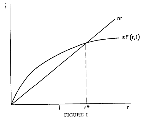
Easy to see that if the production function is increasing and diminishing and shaped as the figure above, then the interaction \(k^*\) would be a stable value (easy to show by discussing before \(k^*\) and after. e.g. if before k* then \(\dot{k}>0\), there is the accumulation of capital per capita).
When\( \frac{\dot{k}}{k} =0\), then \( \frac{\dot{K}}{K} = \frac{\dot{L}}{L}=n\). The implication is that at \(k^*\) (two lines interact, and make \( \frac{\dot{k}}{k} =0\) ) the time-path of labour equal that of capital.
The introduction of Solow (1956) ends there (there are analysis of applying different functional forms of production in his paper, but I would not discuss here), the following are a summary of my previous learning.
P.S. there is no depreciation in the original Solow model.
In summary, the key assumptions are: 1, the law of motion of capital accumulation \(\dot{K}=I\); 2, the shape of the production function.
Solow followed this paper with another pioneering artical, “Technical Change and the Aggregate Production Function.” Before it was published, economists had believed that capital and labour were the main causes of economic growth. But Solow showed that half of economic growth cannot be accounted for by increases in capital and labour.This unaccounted-for portion of economic growth—now called the “Solow residual”—he attributed to technological innovation.
Edmund S. Phelps (new Keynesian) was awarded the 2006 Nobel Prize for the contribution of intertemporal tradeoffs in macroeconomic policy. The intertemporal tradeoffs are from mainly two parts. One is the tradeoff between unemployment and inflation. The other is about capital accumulation and economic growth.
Expectations-Augmented Phillips Curve
In the early 1960s, economists believed that the tradeoff between unemployment and inflation was stable, as the Phillps curve. In the late 1960s, Phelps challenged this view by considering expectation about future inflation.
One of Phelps’ major contributions to economics was the insight he provided on the interaction between inflation and unemployment. In the Expectations-Augmented Phillips curve, he combines current inflation with future inflation and unemployment.
Previous economists including Milton Friedman and Ludwig von Mises argued that people adapt their inflation expectations to account for the effects of expansionary monetary, Phelps is recognised as the first to formally model this phenomenon.
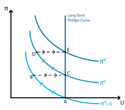
In the first period, the government decides to conduct an expansionary monetary policy, inflation would rise and unemployment would fall, based on the simply Phillps curve. However, a second or third time comes, agents would be quick to associate higher inflation with rising salaries in their expectation adjustment. That would anticipate that inflation would drain their purchasing power accordingly, and the monetary policy would have little effect.
A better way of helping low-skill workers is to expand the earned income tax credit, making it more available to more workers. This way would be more superior to the minimum wages.
The long term Phillips curve is vertical because of the potential GDP. The price level keeps increasing as the expansionary monetary policy. The unemployment rate decrease when the policy is released but the effects diminish in the long run.
Intuitively, if the Federal Reserve increased the money supply at a rate that caused a 5% inflation rate, then, with this higher inflation rate, wages offered would be higher than expected also. Unemployed workers looking for work would see wages that they would mistakenly think were higher in real terms and would, therefore, accept jobs at these wages sooner than otherwise. Millions of unemployed workers taking jobs just a few weeks earlier would result in a lower unemployment rate. Then, however, workers’ expectations would be adaptive; that is, they would adjust to reality. They would realize that the wages weren’t as high in real terms as they had thought, and some would quit and look for more lucrative work, thus slowly raising the unemployment rate. In other words, policymakers could temporarily reduce the unemployment rate by making inflation higher than people expected, but they could not achieve a long-run reduction in unemployment with an increase in inflation. In the long run, then, there is no tradeoff between inflation and unemployment. This striking finding is now mainstream economic wisdom.
Related to Robert Lucas’ work: Lucas emphasised “rational expectations” rather than “adaptive expectations”. The idea is that people would try to anticipate the future based on how the monetary authorities had acted in similar circumstances in the past. In this case, Lucas found even stronger results. Lucas’s model implied that the only way that policymakers could use monetary policy to affect the unemployment rate was by being unpredictable.
Golen Rule
Phelps developed the golden rule of the intertemporal tradeoff between present and future consumption as it relates to capital investment and growth. Phelps’s model formally defines the rate of savings and investment that is necessary to create the maximum level of sustained consumption across successive generations.
In the early 1960s, he derived the “Golden Rule” of capital formation. The rule is that if one’s goal is to attain the maximum consumption per capita that is sustainable in the long run, annual saving as a percent of national income should equal capital’s income as a percent of national income.
In the late 1960s, Phelps did further work in this area with Robert Pollak. They argued that the government should force people to save more than they wish, on the grounds that people put too little weight on their children’s well-being. It seems that the political system, though, does the opposite, especially at the federal level. The federal government taxes the politically powerless younger generation to subsidize—through Medicare and Social Security—today’s politically powerful elderly.
Robert Lucas is a new classical economist and is a Nobel Prize winner in 1995 for developing the theory of rational expectations. He is best known for his development of rational expectations theory and the Lucas critique of macroeconomic policy. Lucas’ study mainly focuses on the implications of the rational expectations theory in macroeconomics.
Theory of Rational Expectations
A vertical Phillips Curve implies that expansionary monetary policy will increase inflation, without boosting the economy. However, Lucas argued that if individuals in the economy are rational, then only unanticipated changes to the money supply will have an impact on output and employment. Otherwise, people will just rationally set their wage and price demands according to their expectations of future inflation as soon as a monetary policy is announced and the policy will only have an impact on prices and inflation rates. In this case, the Phillips Curve is not only vertical in the long run, but also in the short run if policy maker makes unannounced and unpredictable policies.
Lucas Critiques
The Lucas critique, named for Robert Lucas’ work on macroeconomic policymaking, argues that it is naive to try to predict the effects of a change in economic policy entirely on the basis of relationships observed in historical data, especially highly aggregated historical data.
The economic condition is formed by consumer, business, and investor’s behaviours (expectations) based on past data. Expectations will not hold policy changes.
Given that the structure of an econometric model consists of optimal decision rules of economic agents, and that optimal decision rules vary systematically with changes in the structure of series relevant to the decision maker, it follows that any change in policy will systematically alter the structure of econometric models.
Robert Lucas
In other words, changes in a certain factor would affect other factors as well. For example, the government increase tax would result in changes in other economic factors by affecting people’s expectations.
The suggestion of Lucas Critique is that if we want to predict the effect of a policy experiment, we should model the “deep parameters” (relating to preferences, technology and resource constraints) that govern individual behaviour. We can then predict what individuals will do, taking into account the change in policy, and then aggregate the individual decisions to calculate the macroeconomic effects of the policy change.
The Lucas critique was influential not only because it cast doubt on many existing models, but also because it encouraged macroeconomists to build micro-foundations for their models. Microfoundations had always been thought to be desirable; Lucas convinced many economists they were essential. Real Business Cycle economists, starting with Finn Kydland and Edward Prescott, focused their research on using micro-foundations to formulate macroeconomic models. Contemporary macroeconomic models micro-founded on the interaction of rational agents are often called dynamic stochastic general equilibrium (DSGE) models.
Additional
The Lucas Critiques criticised the idea of Keynesian economics that treat the economy as a machine, and apply fiscal and monetary policy to affect the economic operations. Instead, the public sector should consider how private sectors actively react to the policy. For example, if the policy-making (monetary policy such as changes in the interest rate and wage rates) is forecasted by private sectors, then the impacts would be eliminated or reduced, because private sectors would react to the changes by e.g. saving.
Lucas considered that the reason the Keynesian policy works in the short run is there are too many noises in the markets so that private sectors cannot make rational expectations.
That implies the consumption as a ratio over time is a constant, depending on \(\beta, r, \sigma\). Also, as \(\beta (1+r)\) is a very small number, \(ln(\beta (1+r))\approx \beta(1+r)\). Thus, \(\frac{c_t}{c_{t+1}}<0\).
In microeconomics, we always think of factors that grow constantly over time, e.g. constant saving rate.
The “unpleasant arithmetic” stated that if the government has leadership, it can coerce expansions in money.
In contrast, FTPL says that the above restrictions are not a constraint to the CB or government. Instead, it is an equilibrium relation.
As a consequence, the CB and the government may choose policies independent of the above constraint. In the end, the price level \(p_t\) must then adjust such that the equation holds.
Here, I would apply the equation of exchange and government budget constraint to explain how inflation is generated by government deficits. Recalling the government budget constraint,
By denoting real government debt as \( \hat{d}_t=\frac{d_t}{p_{t-1}}\), and replace \( (1+r_t)=(1+i_t)\frac{P_{t-1}}{P_t}=\frac{1+i_t}{1+\pi_t} \) and \( m_t = p_t y_t \), then we get all variables are in real terms,
At the steady state \( g_t=g_{t+1}=g, \tau_t=\tau_{t+1}=\tau \) and so on, and thus,
$$ \underbrace{g+r\hat{d}-\tau }_{Growth\ of \ interest\ deficits}= \underbrace{\frac{p_t-p_{t-1}}{p_t}}_{Seignorage} \times y$$
From the above equation, we can find that if inflation increases then it means the RHS increases. The LHS consists of two parts. Government Spendings \( g + r\hat{d}\) and government revenues \( \tau \). That means the government is getting deficits if the LHS rises. Meanwhile, the RHS increases and so inflation grows.
In sum, we find that government deficits, in the long run, would induce inflation. The zero-inflation condition is to make the LHS of the equation equal to zero (government spendings offset government revenue).
Now assume that money supply follows \(M_{t+1}=(1+\mu)M_t\). Also assume government spending is zero, so all seignorage is redistributed as a (negative) lum-sum tax. ENdowments are constant and given by \(y\).
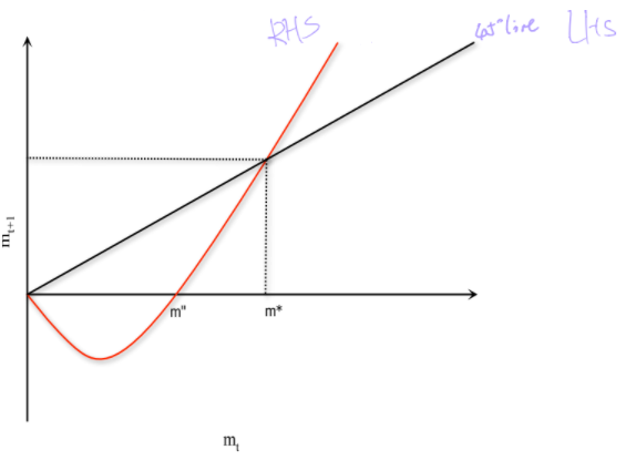
If \( \lim_{m\rightarrow 0}v'(m)m=0\), then \(m^*=0\) is also a steady state equilibrium.
P.S. \(u'(y)=v'(m”)\)
In addition, there exists an \(m”>0\) such that
$$ u'(y)=v'(m”) $$
which implies that \(m_{t+1}\leq0\) for \(m_t\leq m”\).
The relationship could be expressed by the figure below.
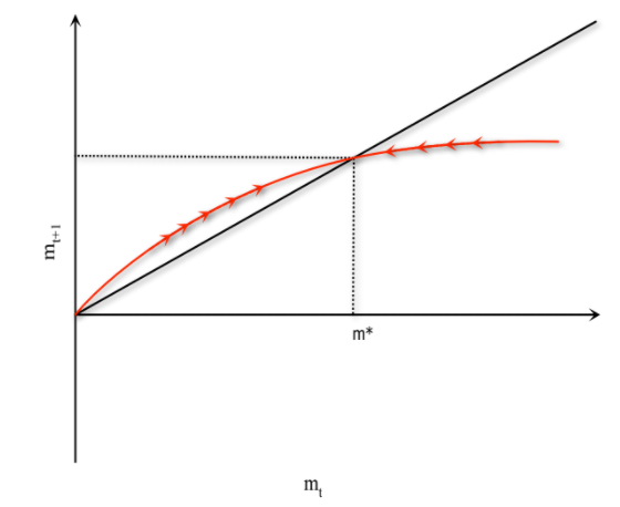
If the initial condition of \(m_t\) is at the right of \(m^*\), then RHS is always greater than the LHS and would result in \(\lim_{t \rightarrow \infty} m_t \rightarrow \infty\). No steady state and violate the transversality condition. Thus, \(m_0\) cannot be at the right of \(m^*\).
If the \(m_0\) at the left of \(m^*\), then \(m_t\) would converge to 0 (as the similar logic above). Therefore, as \(m_t \rightarrow 0\), \(p_t\ rightarrow \infty\) even if \(M_t\) keeps constant. That would lead to hyperinflation.
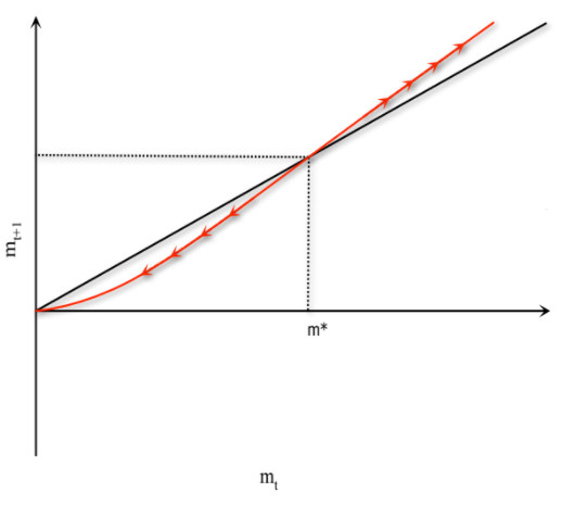
In that scenario, the unique equilibrium is \(m_t=m^*>0\), the price level is determined. Prices, in this case, must be growing at precisely the same rates as money, which adhere to the monetarist doctrine. However, the economy can also display speculative hyperinflation in which inflation far outpace money growth.
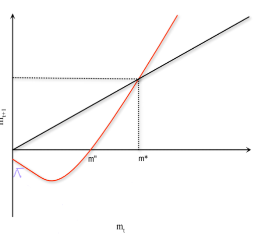
In addition, different forms of the RHS might lead to different results.
E.G. the concavity of RHS, the interaction point at zero, etc would all affect the equilibrium condition.