Surprised Finding from the Book-Thinking, Fast and Slow

Currently, I am reading a book, Thinking, Fast and Slow, which is written by Daniel Kahneman. In this book, the author mentioned a person called Amos several times. As I am pretty interested in the findings and statements in this book, I went to search for who Amos is.

A report caught my eye.

https://www.newyorker.com/books/page-turner/the-two-friends-who-changed-how-we-think-about-how-we-think

That report is written by Cass R. Sunstein and Richard Thaler, two famous psychologists or behaviour economists. Especially, Professor Thaler, if my remembering is not wrong, aroused many ideas about behavioural economics and won the Nobel Prize as well. In this report, they mentioned their Two Friends Who Changed How We Think About How We Think, and their friends clearly are Daniel and Amos.

I am pretty surprised that I find the connection between those famous and legendary economists and psychologists, and decide to keep digging in their previous studies.

Lagrange Multiplier

Here is a review of the method of Lagrangian method. We find that maximising a utility function s.t. a budget constant by using Lagrangian could also get the MRS.

$$\max_{x,y} U(x,y)\quad s.t.\quad BC$$

Or, in a Cobb-Douglas utility.

$$\max_{x,y} x^a y^b\quad s.t.\quad p_x x+p_y y\leq w $$

Using the Lagrange Multiplier,

$$\mathcal{L}=x^a y^b +\lambda (w-p_x x- p_y y)$$

Discuss the complementary slackness, and take F.O.C.

$$ \frac{\partial \mathcal{L}}{\partial x}=0 \Rightarrow a x^{a-1}y^b=\lambda p_x $$

$$ \frac{\partial \mathcal{L}}{\partial y}=0 \Rightarrow x^a b y^{b-1}=\lambda p_y $$

Divide those two equations then we get,

$$ \frac{MU_x}{MU_y}=\frac{ay}{bx}=\frac{p_x}{p_y}=MRS_{x,y} $$

After knowing the Marshallian Demandm \(x=f(p_x,p_y,w)\), we can then calculate the elasticity.

  • \(\varepsilon=\frac{\partial x}{\partial p_x}\frac{p_x}{x}\), elasticity to price of x.
  • \(\varepsilon_I=\frac{\partial x}{\partial w}\frac{w}{x}\), elasticity to wealth.
  • \( \varepsilon_{xy}=\frac{\partial x}{\partial p_y}\frac{p_y}{x} \), elasticity to price of y.

Meaning of Lambda

Review the graphic version of the utility maximisation problem, the budget constraint is the black plane, the utility function is green, and the value of utility is the contour of the utility function.

After solving the utility maximisation problem, we would get \(x^*\) and \(y^*\) (they have exact values). Then, plug them back into the F.O.C., we get easily get the numerical value of \(\lambda\).

As \(\frac{\partial \mathcal{L}}{\partial w}=\lambda\), \(\lambda\) represents how does the utility changes if wealth changes a unit.

\(\lambda\) is like the slope of the utility surface. With the increase, the wealth, the budget constraint (the black wall) moves outwards, and then the changes would result in an increase of the utility value, which is the intersection of the utility surface and the budget constraint surface.

Similarly, the utility function could be replaced with production and has a similar implication of output production.

Geographical Meaning

\(\lambda\) is when the gradient of the contour of the utility function is in the same direction as the gradient of constraint. Or says, the gradient of \(f\) is equal to the gradient of \(g\).

In another word, the Lagrange multiplier \(\lambda\) gives the max and min value of \(x\) and \(y\), and also the corresponding changing speed of those max or mini values of our objective function, \(f\), if the constraint, \(g\), releases.

Lagrange Multiplier:

Simultaneously solve \(\nabla f=\lambda\nabla g\), and \(g=0\). \(f\) here is the objective function (utility function in our case), and \(g\) here is the constraint (the budget constraint in our case).

Reference

Thanks to the video from Professor Burkey, that helps a lot to let me rethink the meaning of lambda.

https://www.youtube.com/watch?v=O3MFXT7AdPg

And the geographic implication of Lagrange multiplier method.

https://www.youtube.com/watch?v=8mjcnxGMwFo

MRS and MRTS

Derivations

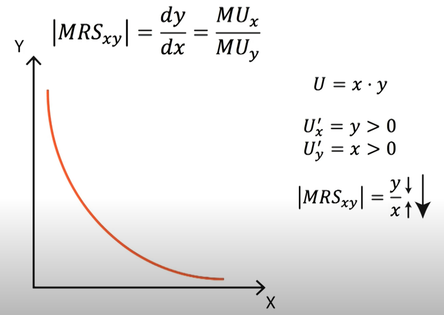
We here derive why \(MRS_{x,y}=\frac{MU_x}{MU_y}\).

Let \(U(x,y)=f(x,y)\), and we know, by definition, MRS measures how many units of x is needed to trade y holding utility constant. Thus, we keep the utility function unchanged, \(U(x,y)=C\), and take differentiation and find \(-dy/dx\).

$$f(x,y) dx=C dx$$

$$ \frac{\partial f(x,y)}{x}+\frac{\partial f(x,y)}{\partial y}\frac{\partial y}{\partial x}=0 $$

$$\frac{\partial y}{\partial x}=-\frac{\frac{\partial f(x,y)}{\partial x}}{\frac{\partial f(x,y)}{\partial y}}=\frac{MU_x}{MU_y}$$

Therefore,

MRS_{x,y}=-\frac{dy}{dx}=\frac{MU_x}{MU_y}

$$|MRS_{x,y}|=-\frac{dy}{dx}=\frac{MU_x}{MU_y} $$

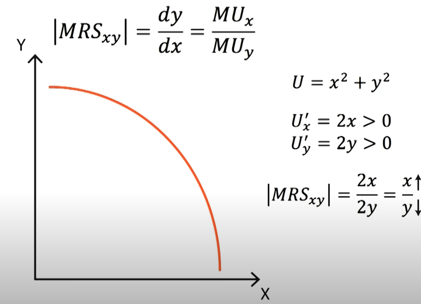
Example 1

$$U=x^2+y^2$$

$$MRS_{x,y}=\frac{MU_x}{MU_y} =\frac{x}{y}$$

Example 2

$$U=x\cdot y$$

, which is similar as the Cobb-Douglas form but has exponenets zero.

$$MRS_{x,y}=\frac{MU_x}{MU_y} =\frac{y}{x}$$

Example 3

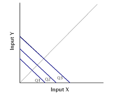
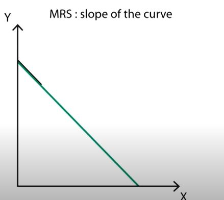
Perfect Substitution: MRS constant
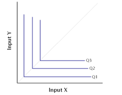
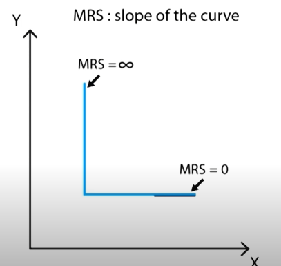
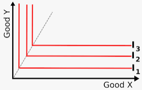
Perfect Complement

MRTS

Marginal Rate of Technical Substitution (MRTS) measures the amount of cost which a specific input can be replaced for another resource of production while maintaining a constant output.

$$MRTS_{K,L}=-\frac{\Delta K}{\Delta L}=-\frac{d K}{d L}=\frac{MP_L}{MP_K}$$

How to derive that?

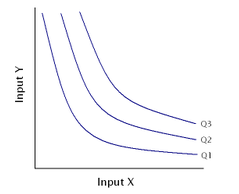
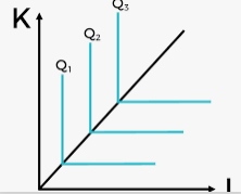
Recall the Isoquant that is equivalent to the contour line of the output function. MRTS is like the slope of the isoquant line. We let,

$$Q=L^a K^b$$

Then,

$$MP_K=\frac{\partial Q}{\partial K}=b L^A K^{b-1}$$

$$MP_L=\frac{\partial Q}{\partial L}=a L^{a-1}K^b$$

$$MRTS=\frac{ b L^A K^{b-1} }{ a L^{a-1}K^b }=\frac{aK}{bL}$$

In short, MRTS is a similar concept to MRS, but in the output aspect.

Cobb-Douglas Function

Cobb-Douglas Utility function

$$U=C x^a y^b$$

While applying the Cobb-Douglas formed utility function, we are actually proxy the preference of people. (The utility function is like a math representation if individuals’ preference is rational). In the utility function, we are focusing more on the Marginal Rate of Substitution between goods.

$$MRS_{x,y}=\frac{MU_x}{MU_y}=\frac{\partial U/\partial x}{\partial U/\partial y}=\frac{Cax^{a-1}y^b}{Cx^a by^{b-1}}$$

$$MRS_{x,y}=\frac{ay}{bx}$$

P.S. Cobb-Douglas gives the same MRS to CES utility function. While solving the utility maximisation problem, we take partial derivatives to the lagrangian and then solve them. Those steps are similar to calculating the MRS.

The key is that the number or value of the utility function does not matter, but the preference represented by the utility function is more important. Any positive monotonic transformation will not change the preference, such as logarithm, square root, and multiply any positive number.

Exponents Do Not Matter

The powers of the Cobb-Douglas function does not really matter as long as they are in the “correct” ratio. For example,

$$ U_1=Cx^7y^1,\quad and \quad U_2=Cx^{7/8}y^{1/8} $$

$$MRS_1=\frac{7y}{x}\quad and \quad MRS_2=\frac{7y/8}{x/8}=\frac{7y}{x}$$

Therefore, we can find that those two utility functions represent the same preference!

Or we can write \(U_1=(U_2)^8 \cdot C^{-7}\). Both taking exponent and multiplying a positive constant are positive monotonic transformations. Therefore, the powers of Cobb-Douglas do not really matter to represent the preference. (\(U=Cx^a y^{1-a}\) the exponents of the utility function does not have to be sum to one).

$$U=x^a y^b \Leftrightarrow x^{\frac{a}{a+b}}y^{\frac{b}{a+b}}$$

Constant Elasticity of Substitution

CES could be either production or utility function. It provides a clear picture of how producers or consumers choose between different choices (elasticity of substitution).

CES Production

The two factor (capital, labour) CES production function was introduced by Solow and later made popular by Arrow.

$$Q=A\cdot(\alpha K^{-\rho}+(1-\alpha)L^{-\rho})^{-\frac{1}{\rho}}$$

  • \(\alpha\) measures the relative proportion spent across K and L.
  • \(\rho=\frac{\sigma-1}{\sigma}\) is the substitution parameter.
  • \(\sigma=\frac{1}{1-\rho}\) is the elasticity of substitution.

While identical producers maximise their profits and markets get competitive, Marginal Product of Labour and Marginal Product of Capital follow,

$$MP_L=\frac{\partial Q}{\partial L}=w$$

$$MP_K=\frac{\partial Q}{\partial K}=r$$

So we get,

$$ \frac{w}{r}=\frac{1-\alpha}{\alpha}(\frac{K}{L})^{\rho+1} $$

$$\frac{K}{L}=(\frac{\alpha}{1-\alpha}\frac{w}{r})^{\frac{1}{1+\rho}}$$

Here, we get the substitution of K and L is a function of the price, w & r. As we are studying the elasticity of substitution, in other words how W/L is affected by w/r, we take derivatives later. We denote \(V=K/L\), and \(Z=w/r\). Then,

$$V=(\frac{\alpha}{1-\alpha}Z)^{\frac{1}{1+\rho}}$$

The Elasticity of Substitution (the percentage change of K/L in terms of the percentage change of w/r) is,

$$ \sigma=\frac{dV/V}{dZ/Z}=\frac{dV}{dZ}\frac{Z}{V}=\frac{1}{1+\rho} $$

Therefore, we get the elasticity of substitution becomes constant, depending on \(\rho\). The interesting thing happens here.

  • If \(-1<\rho<0\), then \(\sigma>1\).
  • If \(0<\rho<\infty\), then \(\sigma<1\).
  • If \(\rho=0\), then, \(\sigma=1\).

Utility Function

Marginal Rate of Substitution (MRS) measures the substitution rate between two goods while holding the utility constant. The elasticity between X and Y could be defined as the following,

$$ Elasticity=\frac{\%\Delta Y}{\% \Delta X}=\frac{\Delta Y/Y}{\Delta X/X}=\frac{X/Y}{\Delta X/\Delta Y} $$

The elasticity of substitution here is defined as how easy is to substitute between inputs, x or y. In another word, the change in the ratio of the use of two goods w.r.t. the ratio of their marginal price. In the utility function case, we can apply the formula,

$$\sigma=\frac{\Delta ln(X/Y)}{\Delta ln(MRS_{X,Y})}=\frac{\Delta ln(X/Y)}{\Delta ln(U_x/U_y)}= \frac{\Delta ln(X/Y)}{\Delta ln(U_x/U_y)} $$

$$\sigma=\frac{\frac{\Delta(X/Y)}{X/Y}}{\frac{\Delta (p_x/p_y)}{p_x/p_y}}$$

  • \(U_x=\frac{\partial U}{\partial X}=p_x\)
  • \(MRS_{X,Y}=\frac{dy}{dx}=\frac{U_x}{U_y}=p_x/p_y\) marginal price in equilibrium.

In the

$$ u(x,y)=(a x^{\rho}+b y^{\rho})^{1/\rho} $$

$$\sigma=\frac{1}{1-\rho}$$

If \(\rho=1\), then \(\sigma\rightarrow \infty\).

If \(\rho\rightarrow -\infty\), then \(\rho=0\).

Two common choices of CES production function are (1) Walras-Leontief-Harrod-Domar function; and (2) Cobb-Douglas function (P.S. but CES is not perfect, coz sigma always equal one).

As \(\rho=1\), the utility function would be a perfect substitute.

As \(\rho=-1\), the utility function would be pretty similar to the Cobb-Douglas form.

Later, the CES utility function could be applied to calculate the Marshallian demand function and Indirect utility function, and so on. Also, easy to show that the indirect utility function \(U(p_x,p_y,w)\) is homogenous degree of 0.

Reference

Arrow, K.J., Chenery, H.B., Minhas, B.S. and Solow, R.M., 1961. Capital-labor substitution and economic efficiency. The review of Economics and Statistics43(3), pp.225-250.

Ideas about Irrational Market Modelling

Continue with the idea that markets are uncompetitive. At the micro-level, the market is constituted by rational players, which takes proportion \(p\) and irrational ones, \(1-p\). They together make the whole market unresponded.

  • A potential study may focus on (1). the drivers of \(p\). (2). modelling the irrational market, establishing a model from micro to macro.
  • For (1), positive feedback or negative feedback may behave differently. Need some psychological knowledge and natural experiment.
  • Using how does market react to positive or negative shocks to distinguish the irrational proportion of people.

Causal Inference in Statistics

Base: Correlation does not mean casualty.

  • If X and Y are statistically dependent, X does not necessarily cause Y (or Y cause X). 相关性不代表有因果性
  • If X causes Y, then X & Y are very likely to be statistically dependent (but not always, there is extreme condition). 但是因果性代表相关性

Study 1. V Structure:

  • Chain

$$ X\rightarrow Y\rightarrow Z $$

Z and X are likely dependent. However, Z and X are independent, conditional on Y.

$$ P(Z=z|X=x,Y=c)=P(Z=z|Y=c) $$i.e.

i.e.

\(f_x: X=u_x\)

\(f_y: Y=84-X+u_Y := c\)

\(f_z: Z=100\underbrace{Y}_{c}+u_z\)

Now, Z and X are independent.

Therefore, we know, in the Chain:

$$ X\equiv Z$$

$$ X\bot Z|Y $$

  • Folk

$$ Y\leftarrow X\rightarrow Z $$

Y and Z are likely dependent. However, Y and Z are independent conditional on X.

$$P(Z=z|Y=y, X=c)=P(Z=z|X=c)$$

While conditioning on intermediate node X, then Z and Y are independent.

$$Y\bot Z|X$$

  • Collider

$$ X\rightarrow Z\leftarrow Y $$

X and Y are independent. However, X and Y are dependent conditional on Z.

$$ P(X=x|Y=y, Z=c)\neq P(X=x|Z=c) $$

i.e.

If we know \(Z=X+Y+u_Z:=c\), then \( X=c-Y-u_Z\), and thus X and Y become dependent conditional on \(Z=c\). Otherwise, \(X=u_X\) and \(Y=u_Y\).

Once, conditioning on \(Z\), the way gets connected. Otherwise (unconditional), we get independent.

P.S. Descendent of Z:

$$ X (or\ Y)\rightarrow Z\rightarrow W $$

Similarly, we get in the Collider:

$$ X\bot Y $$

$$ X\equiv Y|Z $$

$$ X\equiv Y |W $$

  • See notes for further studies.

Reference

Pearl, J., Glymour, M. and Jewell, N.P., 2016. Causal inference in statistics: A primer. John Wiley & Sons.

退休感言-孙振耀(HP大中华区总裁)

职业生涯就像一场体育比赛,有初赛、复赛、决赛。初赛的时候大家都刚刚进社会,大多数都是实力一般的人,这时候努力一点认真一点很快就能让人脱颖而出,于是有的人二十多岁做了经理,有的人迟些也终于赢得了初赛,三十多岁成了经理。然后是复赛,能参加复赛的都是赢得初赛的,每个人都有些能耐,在聪明才智上都不成问题,这个时候再想要胜出就不那么容易了,单靠一点点努力和认真还不够,要有很强的坚忍精神,要懂得靠团队的力量,要懂得收服人心,要有长远的眼光……看上去赢得复赛并不容易,但,还不是那么难。因为这个世界的规律就是给人一点成功的同时让人骄傲自满,刚刚赢得初赛的人往往不知道自己赢得的仅仅是初赛,有了一点小小的成绩大多数人都会骄傲自满起来,认为自己已经懂得了全部,不需要再努力再学习了,他们会认为之所以不能再进一步已经不是自己的原因了。虽然他们仍然不好对付,但是他们没有耐性,没有容人的度量,更没有清晰长远的目光。

职业生涯要关注自己想要什么。人都是要面子的,也是喜欢攀比的,即使在工作上也喜欢攀比,不管那是不是自己想要的。但是攀比并非是好的。

好工作,应该是适合你的工作,具体点说,应该是能给你带来你想要的东西的工作,你或许应该以此来衡量你的工作究竟好不好,而不是拿公司的大小,规模,外企还是国企,是不是有名,是不是上市公司来衡量。

我还是过普通人的日子,要普通人的快乐,至少,晚上睡得着觉。

工作是一件需要理智的事情,所以不要在工作上耍个性。你所在的公司并没有那么烂,你认为不错的公司也没有那么好。35岁以前我们的生存资本靠打拼,35岁以后生存的资本靠的就是积累,这种积累包括人际关系,经验,人脉,口碑……

一份工作到两三年的时候,大部分人都会变成熟手,这个时候往往会陷入不断的重复,有很多人会觉得厌倦,有些人会觉得自己已经搞懂了一切,从而懒得去寻求进步了。很多时候的跳槽是因为觉得失去兴趣了,觉得自己已经完成比赛了。其实这个时候比赛才刚刚开始

并不是你的每一份努力都会得到回报,并不是你的每一次坚持都会有人看到,并不是你每一点付出都能得到公正的回报,并不是你的每一个善意都能被理解……这个,就是世道。好吧,世道不够好,可是,你有推翻世道的勇气么?如果没有,你有更好的解决办法么?有很多时候,人需要一点耐心,一点信心。每个人总会轮到几次不公平的事情,而通常,安心等待是最好的办法。

逆境,是上帝帮你淘汰竞争者的地方。要知道,你不好受,别人也不好受,你坚持不下去了,别人也一样,千万不要告诉别人你坚持不住了,那只能让别人获得坚持的信心,让竞争者看着你微笑的面孔,失去信心,退出比赛。胜利属于那些有耐心的人。

第一件是入行,第二件事情是跟人。要做对的事情,不要让自己今后几十年的人生总是提心吊胆,更不值得为了一份工作赔上自己的青春年华。

好的领导的标准: 首先,好领导要有宽广的心胸,忍住脾气,忍得了比自己强的人;其次,领导要愿意从下属的角度来思考问题,这一点其实是从面试的时候就能发现的,如果这位领导总是从自己的角度来考虑问题,几乎不听你说什么,这就危险了。第三,领导敢于承担责任,如果出了问题就把责任往下推,有了功劳就往自己身上揽,这样的领导不跟也罢。

多认识一些人,多和比自己强的人打交道,同样能找到好的老师,不要和一群同样郁闷的人一起控诉社会,控诉老板,这帮不上你,只会让你更消极。和那些比你强的人打交道,看他们是怎么想的,怎么做的,学习他们,然后跟更强的人打交道。

公司小的时候是销售主导公司,而公司大的时候是财务主导公司,销售的局限性在于只看人情不看数字,财务的局限性在于只看数字不看人情。

人生的三个阶段:一个阶段是为现实找一份工作,一个阶段是为现实,但可以选择一份自己愿意投入的工作,一个阶段是为理想去做一些事情。

近期经济情况 Omicron

  • 当前报道表面Omicron杀伤力较弱。结合其传染力强的特点,有可能帮助全球实现群体免疫。由此US市场普遍对pandemic的预期减弱。
  • 目前Fed政策急转向收紧流动性,减少印钞并加息。市场普遍认为是因为目前美国高通胀。CPI创31年新高(此前是oil crisis)。但是potential reason是,美国就业市场以近饱和,近full employment。继续宽流动性刺激就业会导致hyperinflation。

可以看到labour force participant rate underwent a continuous decrease since 2000. It dropped to the bottom during the pandemic in April 2020 and recovered with the stimulation of public sectors’ policy. However, if taking data before the pandemic, and estimating the decreasing trend (i.e. regress labour force participation rate on time), the forecasted value till current period is about the current value.

That finding implies the labour market has already recovered to the pre-pandemic level. The low level of the labour force participation rate might be that older people do not want to participate in the labour market again and waiting to retire. This implication is also backed by the fact of relatively low level of the unemployment rate.

P.S. there is a negative correlation between the unemployment rate and the federal fund rate. The federal fund rate hikes while the unemployment rate decreases. I would consider that Fed conducts contractionary monetary policy while the economy is close to full employment, controlling the economy not to be overheated.

Based on that, we can find that the Fed calling back the liquidity by increasing interest rate is reasonable. Predict that the Fed would hold a higher federal fund rate, decreasing liquidity and absorbing capital flowing back to the U.S.

Let’s think TAPER and federal fund rate increase together. With an increase in the interest rate in the U.S., money would pour into the U.S. pursuing higher interest rate payments. People would therefore sell assets from other countries for money, resulting in a decrease in the capital market.

中央经济局会议 2021.12.08-10

会议指出在充分肯定成绩的同时,必须看到我国经济发展面临需求收缩、供给冲击、预期转弱三重压力

会议要求,明年经济工作要稳字当头、稳中求进,各地区各部门要担负起稳定宏观经济的责任,各方面要积极推出有利于经济稳定的政策,政策发力适当靠前。

  • 1. 宏观政策要稳健有效。要继续实施积极的财政政策和稳健的货币政策。积极的财政政策要提升效能,更加注重精准、可持续。要保证财政支出强度,加快支出进度。实施新的减税降费政策,强化对中小微企业、个体工商户、制造业、风险化解等的支持力度,适度超前开展基础设施投资。党政机关要坚持过紧日子。严肃财经纪律。坚决遏制新增地方政府隐性债务。稳健的货币政策要灵活适度,保持流动性合理充裕。引导金融机构加大对实体经济特别是小微企业、科技创新、绿色发展的支持。财政政策和货币政策要协调联动,跨周期和逆周期宏观调控政策要有机结合。实施好扩大内需战略,增强发展内生动力。

通过fiscal policy:减tax增加Government spending着重刺激小企业=>目的为刺激地方经济发展,且为带动就业(需考虑提高市场主体带动就业的能力)。

通过monetary policy:释放流动性,支持实体经济小微企业进行科技创新。

  • 2. 微观政策要持续激发市场主体活力。要提振市场主体信心,深入推进公平竞争政策实施,加强反垄断和反不正当竞争,以公正监管保障公平竞争。强化知识产权保护,营造各类所有制企业竞相发展的良好环境。强化契约精神,有效治理恶意拖欠账款和逃废债行为。

微观层面增强市场的竞争水平,反垄断(此点需要结合支持小企业发展才能支持企业之间进行竞争)。提高社会主体及企业公信度,减少违约行为发生。

  • 3. 结构政策要着力畅通国民经济循环。要深化供给侧结构性改革,重在畅通国内大循环,重在突破供给约束堵点,重在打通生产、分配、流通、消费各环节。要提升制造业核心竞争力,启动一批产业基础再造工程项目,激发涌现一大批“专精特新”企业。加快形成内外联通、安全高效的物流网络。加快数字化改造促进传统产业升级。要坚持房子是用来住的、不是用来炒的定位,加强预期引导,探索新的发展模式,坚持租购并举,加快发展长租房市场,推进保障性住房建设,支持商品房市场更好满足购房者的合理住房需求,因城施策促进房地产业良性循环和健康发展。

支持供应链改革优化,提高资源产出效率。

支持专精特新,提高我国企业在国际范围的竞争力。

加强数字化转型:提高企业内生产效率

房主不炒,避免房地产市场吸纳过多资金,发展长租房市场

  • 4. 科技政策要扎实落地。要实施科技体制改革三年行动方案,制定实施基础研究十年规划。强化国家战略科技力量,发挥好国家实验室作用,重组全国重点实验室,推进科研院所改革。强化企业创新主体地位,深化产学研结合。完善优化科技创新生态,形成扎实的科研作风。继续开展国际科技合作。

推动科技发展,同时保证产学研结合,将研究的科技产出应用到企业生产。

  • 改革开放政策要激活发展动力。要抓好要素市场化配置综合改革试点,全面实行股票发行注册制,完成国企改革三年行动任务,稳步推进电网、铁路等自然垄断行业改革。调动地方改革积极性,鼓励各地因地制宜、主动改革。扩大高水平对外开放,推动制度型开放,落实好外资企业国民待遇,吸引更多跨国公司投资,推动重大外资项目加快落地。推动共建“一带一路”高质量发展。

要素市场资源分配。推动电网、铁路等大国企市场化。吸引外资企业注入,吸纳国际资金,解决国内就业。

  • 区域政策要增强发展的平衡性协调性。要深入实施区域重大战略和区域协调发展战略,促进东、中、西和东北地区协调发展。全面推进乡村振兴,提升新型城镇化建设质量。

区域发展不均衡,推动乡村发展

  • 社会政策要兜住兜牢民生底线。要统筹推进经济发展和民生保障,健全常住地提供基本公共服务制度。解决好高校毕业生等青年就业问题,健全灵活就业劳动用工和社会保障政策。推进基本养老保险全国统筹。推动新的生育政策落地见效,积极应对人口老龄化。

就业问题,公共服务问题,社保问题。养老问题。

  1. 把握共同富裕目标。合理资源分配制度,加强社保、税收、转移支付等政策力度;推动高质量发展要以就业为导向;完善公共服务制度体系,教育、医疗、养老、住房等。完善第二次分配和第三次分配的方向。
  2. 加强资本监管,防止资本野蛮生长。
  3. 节约资源利用,推进资源全面节约、集约、循环利用。
  4. 防范风险:行业、企业。
  5. 碳达峰碳中和:技术攻关。早实现能耗“双控”向碳排放总量和强度“双控”转变。保供稳价。